Validating a finite-element crack
How much the corrected boundary condition buys, and how close the finite-element crack gets to the closed form it is meant to reproduce. The method is in The finite Eshelby cell; how to call it is in Finite-element inclusions.
The figures and the numbers are produced once by scripts/fe/make_doc_figures.jl and committed; the live demonstrations are scripts/81_fe_crack_eshelby.jl and scripts/82_fe_crack_schemes.jl.
The correction is the $(a/R)^3$ dipole
$\|\mathbf B_u\|$ measures the truncation bias being removed. If the boundary term really is the elastic dipole, it must fall like the cube of the domain radius — and it does, over a decade:
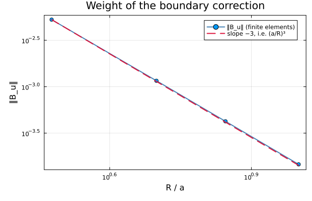
| R/a | ‖B_u‖ |
|---|---|
| 3 | 5.273e-03 |
| 5 | 1.159e-03 |
| 7 | 4.240e-04 |
| 10 | 1.458e-04 |
Fitted log-log slope: −2.98 against a theoretical −3. This is the sharpest available check that the dipole boundary condition has the right magnitude and the right sign — a sign error would not merely change the exponent, it would send $\mathbf B_\infty$ the wrong way.
Note how small the correction is at R = 5a (≈ 0.1 % on B). That is the whole point: it is what makes so small a domain legitimate, at the cost of three extra solves that share the existing factorization.
Convergence to the closed form
The crack front carries a square-root displacement field, so a fixed-order element converges slowly — in practice first order in the element size $h \propto 1/\texttt{htipdiv}$. That regularity is what makes Richardson extrapolation to $h\to 0$ legitimate, and it turns a few-percent raw error into a sub-percent verdict.
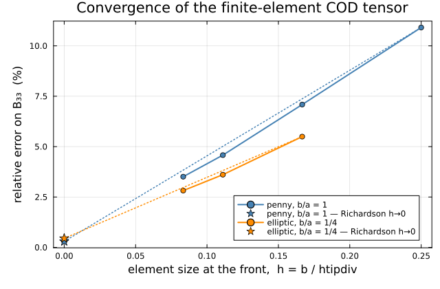
Isotropic matrix, $E = 1$, $\nu = 0.3$, radius_ratio = 5.
Penny-shaped crack (b/a = 1), closed form diag(B) = [1.81749, 1.81749, 1.54486]:
| h at the front | dofs | diag(B) | relative error (%) |
|---|---|---|---|
| b/4 | 14 865 | [1.55789, 1.56444, 1.37630] | [−14.28, −13.92, −10.91] |
| b/6 | 21 954 | [1.65089, 1.65308, 1.43537] | [−9.17, −9.05, −7.09] |
| b/9 | 43 515 | [1.70740, 1.70724, 1.47413] | [−6.06, −6.07, −4.58] |
| b/12 | 86 784 | [1.73522, 1.73483, 1.49067] | [−4.53, −4.55, −3.51] |
| h → 0 (Richardson) | — | [1.81867, 1.81760, 1.54029] | [+0.06, +0.01, −0.30] |
Elliptical crack (b/a = 1/4), closed form diag(B) = [3.09055, 2.33845, 2.26304]:
| h at the front | dofs | diag(B) | relative error (%) |
|---|---|---|---|
| b/6 | 61 941 | [2.91496, 2.14285, 2.13865] | [−5.68, −8.36, −5.50] |
| b/9 | 117 516 | [2.97504, 2.21003, 2.18140] | [−3.74, −5.49, −3.61] |
| b/12 | 220 176 | [2.99958, 2.23898, 2.19927] | [−2.94, −4.25, −2.82] |
| h → 0 (Richardson) | — | [3.07321, 2.32582, 2.25291] | [−0.56, −0.54, −0.45] |
The raw finite-element opening sits a few percent below the closed form, and for two compounding reasons that both push the same way: a truncated cell is stiffer than an infinite medium, and a fixed-order element under-resolves the front. The extrapolated values land within a percent — the residual is discretization, not a modelling error.
For reference, the FEniCSx implementation of the same scheme in the SifAniso study reports ±5 % on $\mathbf B_\infty$ at htipdiv = 12 with P3 elements.
See also
- The finite Eshelby cell — the method
- Finite-element inclusions — the commands
- A recycled-concrete aggregate — the same correction on a solid inclusion, in its general form