An inclusion whose response is a neural network
MeanFieldHom lets a morphology take part in every homogenization scheme provided it can answer one of three questions — the Hill tensor, the localization tensors, or the contribution tensors. Nothing says the answer has to come from a formula. It can come from a finite-element solve (FEEllipticCrack, FEExcenteredSphere), and it can come from a trained network, which is what this script drives.
The morphology here is the ellipsoid, whose Hill tensor is known in closed form. That is the point: it is the one case where a surrogate can be held to an exact answer, so every part of the pipeline — the sampling, the labelling, the decode, the frame conventions, the schemes, the sensitivities — can be checked before being pointed at something unknown.
What a surrogate buys, and what it does not:
| analytic ellipsoid | finite elements | surrogate | |
|---|---|---|---|
| accuracy | exact | discretization error | fit error, a few parts in 10⁴ to 10³ here |
| cost per evaluation | microseconds | seconds | microseconds |
| derivative w.r.t. the morphology | yes | refused | yes |
The middle column is why this exists. A finite-element inclusion cannot be differentiated with respect to an aspect ratio — its solve runs in Float64 and memoizes on the reference medium, so the derivative would come back as a silent zero, and MeanFieldHom.FiniteElements refuses the request outright. A surrogate trained on that same solve is smooth, cheap, and differentiable.
The models are loaded from src/NeuralInclusions/models/, trained once by scripts/nn/train_models.jl. Nothing is fitted here, so this script needs no machine-learning dependency at all.
using MeanFieldHom
using TensND
using LinearAlgebra
using Printf
using Plots

gr()

default(; left_margin = 5Plots.mm, bottom_margin = 5Plots.mm)

const NI = MeanFieldHom.NeuralInclusionsMeanFieldHom.NeuralInclusions§1 The two phases
What the network is
Not much: a three-layer perceptron with smooth activations, wrapped in the algebra that makes the answer a tensor. Everything outside the dashed box is exact and enforced — the standardization, the inverse component transform, and a decode that puts the components into a structured TensND type in the inclusion's own frame, with the dependence on the reference moduli applied analytically. The network is only asked for what is genuinely unknown: how the dimensionless components vary with the shape.
Smooth activations are not a detail: a kink in the activation is a kink in $\mathbb P$, hence a wrong curvature and a discontinuous sensitivity. The activation table offers tanh and softplus and deliberately no ReLU.
How it is trained
The two green boxes are the only morphology-dependent part. response is where a finite-element solve goes instead of a closed form — and because the frame in which the labels are read is derived from geometry through the same code path the inclusion uses at evaluation time, the two cannot disagree.
The call itself, for the record — not run here, since fitting needs Lux, Optimisers and Zygote and this page must not train anything:
import Lux, Optimisers, Zygote                    # activates MeanFieldHomLuxExt

geometry(x) = Ellipsoid(1.0, 1.0, exp(x[1]))      # shape features → morphology
response(g, C₀) = hill_tensor(g, C₀)              # what is to be learned

spec = DimensionlessHill(HillTI())
box = SampleBox([:log_aspect, :nu0], [-log(20), 0.0], [log(20), 0.49])

train, val = generate_dataset(geometry, response, spec, box, 6000; nvalidation = 1500)
s = train_surrogate(spec, box, train, val; teacher_name = "analytic Hill tensor")

report_surrogate(s, val; labels = component_labels(spec))
save_surrogate("my_model.json", s)
scripts/nn/train_models.jl is that script for the four shipped models. It also records the learning curves, which is where this figure comes from:
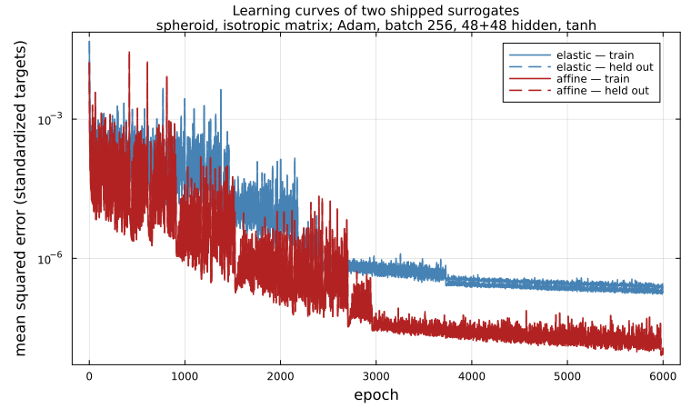
Held-out and training error stay together — a network this small over a two-dimensional box has no room to overfit — and the steps are the plateau schedule dropping the Adam step. The red pair is the AffineHill model, which settles an order of magnitude lower than the blue DimensionlessHill one for the same architecture: it does not spend capacity on a dependence that is exactly known (§5).
§2 The shipped models
Each carries its own provenance: what generated its labels, how many samples, and the per-component error measured on a held-out set. That last number is not decoration — it is what a tolerance should be derived from, here and in the test suite, so that a retraining cannot silently loosen a threshold.
println("shipped surrogates:")
for name in shipped_models()
    s = load_surrogate(model_path(name))
    @printf(
        "  %-32s %-22s worst rel. err %8.2e   (%d train / %d held out)\n",
        name, "(" * join(s.features, ", ") * ")",
        worst_error(s.provenance), s.provenance.nsamples, s.provenance.nvalidation
    )
end

elastic = load_surrogate(model_path("spheroid_hill_iso_elastic"))
conduction = load_surrogate(model_path("spheroid_hill_iso_conduction"))
triaxial = load_surrogate(model_path("triaxial_hill_iso_elastic"))
affine = load_surrogate(model_path("spheroid_hill_iso_affine"))
NeuralSurrogate(log_aspect → :affine/:ti, order 4; MLP(1→48→48→10, tanh, tanh, identity; 2938 params); worst rel. error 2.65e-04)A spheroid in the sorted convention: semi-axes descending, so the aspect ratio that matters is distinct over equal — positive logarithm for a prolate particle, negative for an oblate one, zero for a sphere.
spheroid(ω; kw...) = ω ≥ 1 ? Ellipsoid(ω, 1.0, 1.0; kw...) : Ellipsoid(1.0, 1.0, ω; kw...)

nn_spheroid(ω; kw...) = NeuralHillInclusion(
    spheroid(ω).semi_axes;
    elastic, transport = conduction, guard = :error, kw...
)
nn_spheroid (generic function with 1 method)check_inclusion_interface reports which gate the inclusion satisfies. Gate A — the Hill tensor — is the most complete: the eight localization tensors, the four contribution tensors and every scheme are derived from it.
println()
check_inclusion_interface(nn_spheroid(0.4))true§3 What is exact regardless of the fit
A surrogate should only ever learn what is genuinely unknown. Three properties of the Hill tensor are exact, and all three are enforced by construction rather than fitted — so they hold to machine precision no matter how badly the network is trained.
Zero contrast. Gate A supplies $\mathbb P$, and the package evaluates
\[\mathbb A_{\varepsilon\varepsilon} = \bigl[\mathbb I + \mathbb P : (\mathbb C_1 - \mathbb C_0)\bigr]^{-1}\]
exactly, so $\mathbb C_1 = \mathbb C_0 \Rightarrow \mathbb A = \mathbb I$. The fit error is confined to a single tensor, and the eight localization tensors stay exactly consistent with one another — which a surrogate predicting $\mathbb A$ directly could not guarantee, $\mathbb A$ having no major symmetry.
Homogeneity. $\mathbb P(\lambda\mathbb C_0) = \mathbb P(\mathbb C_0)/\lambda$, so the network never sees an absolute modulus.
Symmetry class and frame. The decoder emits a structured TensND type from the right number of components, in the inclusion's own frame.
C₀ = iso_stiffness(30.0, 10.0)
incl = nn_spheroid(0.4)

A_zero = strain_strain_loc(incl, C₀, C₀)
@printf(
    "\n  |𝔸 − 𝕀| at zero contrast          %.2e\n",
    maximum(abs, get_array(A_zero) .- get_array(TensISO{3}(1.0, 1.0)))
)

P = hill_tensor(incl, C₀)
@printf(
    "  |λℙ(λℂ₀) − ℙ(ℂ₀)| at λ = 17       %.2e\n",
    maximum(abs, 17 .* get_array(hill_tensor(incl, 17 * C₀)) .- get_array(P))
)

Parr = get_array(P)
@printf("  major symmetry of ℙ                %.2e\n", maximum(abs, Parr .- permutedims(Parr, (3, 4, 1, 2))))
println("  class of ℙ                         ", nameof(typeof(P)), " with ", length(get_data(P)), " components")
  |𝔸 − 𝕀| at zero contrast          0.00e+00
  |λℙ(λℂ₀) − ℙ(ℂ₀)| at λ = 17       4.34e-19
  major symmetry of ℙ                0.00e+00
  class of ℙ                         TensTI with 5 components
Rotating the inclusion rotates the tensor and leaves its components alone: the orientation is never an input, so frame indifference is exact too.
rot = nn_spheroid(0.4; euler_angles = (0.3, 0.7, 0.2))
@printf(
    "  |Δcomponents| under a rotation     %.2e\n",
    maximum(abs, collect(get_data(hill_tensor(rot, C₀))) .- collect(get_data(P)))
)
|Δcomponents| under a rotation 0.00e+00§4 Accuracy against the closed form
Over two decades of aspect ratio either side of the sphere, and across the Poisson range. The oblate side is the harder one: several Walpole components grow like $1/\omega$ as the particle flattens, which is why the fit is done on a per-component logarithmic scale where the dynamic range calls for it.
function hill_error(incl_of, exact_of, ω, C)
    Pn = get_array(hill_tensor(incl_of(ω), C))
    Pe = get_array(hill_tensor(exact_of(ω), C))
    return maximum(abs, Pn .- Pe) / maximum(abs, Pe)
end

const OMEGAS = (0.06, 0.1, 0.25, 0.5, 0.9, 1.2, 2.5, 6.0, 18.0)

println("\n  ℙ of a spheroid — relative error against the analytic tensor\n")
println("      ω        ν₀ = 0.05     ν₀ = 0.20     ν₀ = 0.45")
for ω in OMEGAS
    errs = map((0.05, 0.2, 0.45)) do nu
        hill_error(nn_spheroid, spheroid, ω, iso_stiffness_E_nu(1.0, nu))
    end
    @printf("  %7.2f      %9.2e     %9.2e     %9.2e\n", ω, errs...)
end
  ℙ of a spheroid — relative error against the analytic tensor

      ω        ν₀ = 0.05     ν₀ = 0.20     ν₀ = 0.45
     0.06       2.85e-04      1.33e-05      7.46e-04
     0.10       7.37e-04      3.12e-04      6.56e-04
     0.25       8.90e-05      5.10e-05      1.59e-04
     0.50       2.07e-04      4.83e-04      1.65e-04
     0.90       3.14e-04      7.37e-04      3.81e-04
     1.20       6.32e-05      6.24e-05      6.22e-04
     2.50       1.46e-04      3.26e-05      7.87e-05
     6.00       1.50e-04      3.11e-05      1.97e-04
    18.00       3.65e-05      1.08e-04      1.30e-04
The transport tensor is the easy case, and the sharpest check that the decode is right: the second-order Hill tensor is exactly $\mathbb V^{\mathbf A}/k_0$, so the conductivity divides out and the surrogate is a function of the shape alone — one input, no material feature.
K₀ = TensISO{3}(2.0)
println("\n  ℙ_K of a spheroid — no material feature, the 1/k₀ scaling is exact\n")
println("      ω      relative error")
for ω in OMEGAS
    Pn = get_array(hill_tensor(nn_spheroid(ω), K₀))
    Pe = get_array(hill_tensor(spheroid(ω), K₀))
    @printf("  %7.2f      %9.2e\n", ω, maximum(abs, Pn .- Pe) / maximum(abs, Pe))
end
  ℙ_K of a spheroid — no material feature, the 1/k₀ scaling is exact

      ω      relative error
     0.06       3.44e-05
     0.10       5.87e-06
     0.25       3.25e-05
     0.50       1.41e-04
     0.90       8.05e-05
     1.20       8.14e-05
     2.50       1.07e-04
     6.00       3.09e-05
    18.00       1.86e-05
The triaxial ellipsoid asks for nine components from three features. Its parametrization is (a₂/a₁, a₃/a₂) rather than (a₂/a₁, a₃/a₁): with the semi-axes sorted descending, the admissible set of the first pair is exactly a box, while the second is confined to a triangular wedge.
nn_triaxial(r2, r3) = NeuralHillInclusion(
    Ellipsoid(1.0, r2, r3).semi_axes; elastic = triaxial, guard = :error
)

println("\n  ℙ of a triaxial ellipsoid, ν₀ = 0.25\n")
println("    a₂/a₁    a₃/a₁    relative error")
for (r2, r3) in ((0.9, 0.8), (0.8, 0.5), (0.6, 0.2), (0.5, 0.1), (0.2, 0.08))
    C = iso_stiffness_E_nu(1.0, 0.25)
    Pn = get_array(hill_tensor(nn_triaxial(r2, r3), C))
    Pe = get_array(hill_tensor(Ellipsoid(1.0, r2, r3), C))
    @printf("  %7.2f  %7.2f      %9.2e\n", r2, r3, maximum(abs, Pn .- Pe) / maximum(abs, Pe))
end
  ℙ of a triaxial ellipsoid, ν₀ = 0.25

    a₂/a₁    a₃/a₁    relative error
     0.90     0.80       1.84e-03
     0.80     0.50       3.81e-04
     0.60     0.20       2.00e-04
     0.50     0.10       7.91e-05
     0.20     0.08       1.08e-04
§5 Removing ν₀ from the inputs altogether
Nothing new is needed here: it is the shape/moduli factorization the theory page already states for an isotropic matrix,
\[\mathbb P\bigl(\boldsymbol A,\, 3\lambda_0\mathbb I + 2\mu_0\mathbb K\bigr) = \frac{1}{\lambda_0 + 2\mu_0}\,\mathbb U^{\boldsymbol A} + \frac{1}{\mu_0}\bigl(\mathbb V^{\boldsymbol A} - \mathbb U^{\boldsymbol A}\bigr),\]
with the geometric auxiliaries tens_UA and tens_VA — functions of the shape alone. Collecting the two terms,
\[\mathbb P = d\,\mathbb U^{\boldsymbol A} + \frac{1}{\mu_0}\,\mathbb V^{\boldsymbol A}, \qquad d = \frac{1}{\lambda_0 + 2\mu_0} - \frac{1}{\mu_0},\]
which is affine in $(d, 1/\mu_0)$. AffineHill exploits it: the network predicts those two tensors — twice the components, one fewer input — and the decoder contracts them with the exact coefficients, so the entire material dependence becomes algebra.
Nothing shape-specific is reimplemented to get there. Both tensors live in the same symmetry class as $\mathbb P$, so their components are recovered from two teacher evaluations at two Poisson ratios by solving the 2×2 system componentwise.
The consequence is visible in the table below: the generic model, which fits ν₀, degrades towards the incompressible end where $d$ varies fastest, whereas the affine model is flat in ν₀ — it never saw a Poisson ratio at all.
nn_affine(ω) = NeuralHillInclusion(
    spheroid(ω).semi_axes; elastic = affine, guard = :error
)

const NUS = (0.02, 0.15, 0.3, 0.42, 0.48)

println("\n  relative error on ℙ, ω = 0.25 — ν₀ fitted versus ν₀ exact\n")
println("      ν₀      DimensionlessHill    AffineHill")
for nu in NUS
    C = iso_stiffness_E_nu(1.0, nu)
    eg = hill_error(nn_spheroid, spheroid, 0.25, C)
    ea = hill_error(nn_affine, spheroid, 0.25, C)
    @printf("  %7.2f          %9.2e     %9.2e\n", nu, eg, ea)
end
  relative error on ℙ, ω = 0.25 — ν₀ fitted versus ν₀ exact

      ν₀      DimensionlessHill    AffineHill
     0.02           1.91e-04      9.71e-06
     0.15           1.23e-04      1.46e-05
     0.30           2.14e-04      2.67e-05
     0.42           3.27e-04      5.28e-05
     0.48           6.43e-04      7.51e-05
Across the whole box, in one figure: the error against the aspect ratio, for the two factorizations, at the two ends of the Poisson range.
ωs = exp.(range(log(1 / 18), log(18.0); length = 90))
plt = plot(;
    xscale = :log10, yscale = :log10, xlabel = "aspect ratio ω = distinct / equal",
    ylabel = "relative error on ℙ", legend = :bottomright, size = (780, 470),
    title = "Fitted versus exact ν₀ dependence\n" *
        "spheroid, isotropic matrix; both nets 48+48 hidden, 6000 train / 1500 held out",
    titlefontsize = 10,
)
for (nu, col) in ((0.05, :steelblue), (0.48, :firebrick))
    C = iso_stiffness_E_nu(1.0, nu)
    plot!(
        plt, ωs, [hill_error(nn_spheroid, spheroid, ω, C) for ω in ωs];
        lc = col, lw = 2, label = "DimensionlessHill, ν₀ = $nu"
    )
    plot!(
        plt, ωs, [hill_error(nn_affine, spheroid, ω, C) for ω in ωs];
        lc = col, lw = 2, ls = :dash, label = "AffineHill, ν₀ = $nu"
    )
end
plt
§6 In every scheme
Gate A means there is nothing left to implement: the surrogate is a drop-in Ellipsoid, in elasticity and in transport. The inclusion is tilted, so the effective tensor is genuinely anisotropic and a dropped rotation cannot hide behind an isotropic answer.
One caveat, and it is the shipped models' only real restriction: they are trained for an isotropic reference medium — ν₀ is their material feature, and the exact homogeneity used to decode assumes isotropy. The one-shot schemes evaluate the inclusion in the reference medium you supply, so they are unaffected. The iterative ones — SelfConsistent, AsymmetricSelfConsistent, DifferentialScheme — re-evaluate it in their own current estimate, which for a single tilted spheroid is transversely isotropic, and the surrogate refuses it rather than extrapolating silently. symmetrize = IsoSymmetrize() is the answer: the scheme then hands the kernel a pre-projected isotropic reference at every iteration. This is the same restriction the finite-element inclusions carry, for the same reason.
C_M, C_I = iso_stiffness(30.0, 10.0), iso_stiffness(60.0, 20.0)
K_M, K_I = TensISO{3}(2.0), TensISO{3}(7.0)

ell = spheroid(0.4; euler_angles = (0.3, 0.7, 0.0))
nn = NeuralHillInclusion(
    ell.semi_axes; basis = MeanFieldHom.inclusion_basis(ell),
    elastic, transport = conduction, guard = :error
)

function rve_with(geom, prop_m, prop_i, key; kw...)
    r = RVE(:M)
    add_matrix!(r, Ellipsoid(1.0), Dict(key => prop_m))
    add_phase!(r, :I, geom, Dict(key => prop_i); fraction = 0.25, kw...)
    return r
end

c1111(C) = get_array(C)[1, 1, 1, 1]
k11(K) = get_array(K)[1, 1]

println("\n  Elasticity, one-shot schemes — C_eff[1,1,1,1]\n", "-"^62)
@printf "  %-16s %14s %14s %12s\n" "scheme" "Ellipsoid" "surrogate" "rel. Δ"
for (name, sch) in (
        "Dilute" => Dilute(), "DiluteDual" => DiluteDual(),
        "MoriTanaka" => MoriTanaka(), "Maxwell" => Maxwell(),
        "PCW" => PonteCastanedaWillis(),
    )
    ref = c1111(homogenize(rve_with(ell, C_M, C_I, :C), sch, :C))
    got = c1111(homogenize(rve_with(nn, C_M, C_I, :C), sch, :C))
    @printf "  %-16s %14.8f %14.8f %12.2e\n" name ref got abs(got - ref) / abs(ref)
end
  Elasticity, one-shot schemes — C_eff[1,1,1,1]
--------------------------------------------------------------
  scheme                Ellipsoid      surrogate       rel. Δ
  Dilute              50.54177297    50.54299067     2.41e-05
  DiluteDual          52.01312747    52.01485604     3.32e-05
  MoriTanaka          51.18088346    51.18198786     2.16e-05
  Maxwell             51.35179859    51.35331751     2.96e-05
  PCW                 51.35179859    51.35331751     2.96e-05
The iterative schemes, with the isotropic projection that keeps their running reference inside the surrogate's domain. Both columns get the same option, so the comparison is like for like.
println(
    "\n  Elasticity, iterative schemes + IsoSymmetrize — C_eff[1,1,1,1]\n", "-"^62
)
@printf "  %-16s %14s %14s %12s\n" "scheme" "Ellipsoid" "surrogate" "rel. Δ"
for (name, sch) in (
        "SelfConsistent" => SelfConsistent(),
        "ASC" => AsymmetricSelfConsistent(),
        "Differential" => DifferentialScheme(),
    )
    kw = (; symmetrize = IsoSymmetrize())
    ref = c1111(homogenize(rve_with(ell, C_M, C_I, :C; kw...), sch, :C))
    got = c1111(homogenize(rve_with(nn, C_M, C_I, :C; kw...), sch, :C))
    @printf "  %-16s %14.8f %14.8f %12.2e\n" name ref got abs(got - ref) / abs(ref)
end
  Elasticity, iterative schemes + IsoSymmetrize — C_eff[1,1,1,1]
--------------------------------------------------------------
  scheme                Ellipsoid      surrogate       rel. Δ
  SelfConsistent      50.94576661    50.94664639     1.73e-05
  ASC                 50.96083479    50.96201122     2.31e-05
  Differential        50.88806005    50.88918371     2.21e-05
Without it, the refusal is explicit rather than silent — which is the whole point of the domain guard.
try
    homogenize(rve_with(nn, C_M, C_I, :C), SelfConsistent(), :C)
catch e
    println("\n  SelfConsistent without IsoSymmetrize:")
    println("    ", first(split(sprint(showerror, e), ". ")), ".")
end

println("\n  Conduction — K_eff[1,1]\n", "-"^62)
@printf "  %-16s %14s %14s %12s\n" "scheme" "Ellipsoid" "surrogate" "rel. Δ"
for (name, sch) in (
        "Dilute" => Dilute(), "DiluteDual" => DiluteDual(),
        "MoriTanaka" => MoriTanaka(), "Maxwell" => Maxwell(),
    )
    ref = k11(homogenize(rve_with(ell, K_M, K_I, :K), sch, :K))
    got = k11(homogenize(rve_with(nn, K_M, K_I, :K), sch, :K))
    @printf "  %-16s %14.8f %14.8f %12.2e\n" name ref got abs(got - ref) / abs(ref)
end
  SelfConsistent without IsoSymmetrize:
    ArgumentError: the :nu0 feature needs an isotropic reference medium and got a TensTI.

  Conduction — K_eff[1,1]
--------------------------------------------------------------
  scheme                Ellipsoid      surrogate       rel. Δ
  Dilute               2.80888014     2.80885806     7.86e-06
  DiluteDual           3.36763434     3.36756950     1.93e-05
  MoriTanaka           2.88610461     2.88608493     6.82e-06
  Maxwell              2.93612460     2.93609480     1.02e-05
Orientation averaging is applied by the scheme after the surrogate returns, so it costs nothing: a family of orientations under TISymmetrize reproduces the native answer to the surrogate's own accuracy.
function oriented(build, nbins, f)
    r = RVE(:M)
    add_matrix!(r, Ellipsoid(1.0), Dict(:C => C_M))
    for (i, bin) in enumerate(polar_orientation_bins(nbins))
        add_phase!(
            r, Symbol(:I, i), build(bin.θ), Dict(:C => C_I);
            fraction = f * bin.weight, symmetrize = TISymmetrize((0.0, 0.0, 1.0))
        )
    end
    return r
end
ell_at(θ) = spheroid(0.4; euler_angles = (θ, 0.0, 0.0))
nn_at(θ) = let e = ell_at(θ)
    NeuralHillInclusion(
        e.semi_axes; basis = MeanFieldHom.inclusion_basis(e), elastic, guard = :error
    )
end

C_ref = homogenize(oriented(ell_at, 12, 0.2), MoriTanaka(), :C)
C_nn = homogenize(oriented(nn_at, 12, 0.2), MoriTanaka(), :C)
@printf(
    "\n  12 polar bins + TISymmetrize: %s versus %s, max rel. Δ = %.2e\n",
    typeof(C_ref).name.name, typeof(C_nn).name.name,
    maximum(abs, get_array(C_nn) .- get_array(C_ref)) / maximum(abs, get_array(C_ref))
)
12 polar bins + TISymmetrize: TensTI versus TensTI, max rel. Δ = 1.78e-05§7 The derivative with respect to the morphology
This is what the surrogate is really for. A network is a smooth function of its inputs, so ForwardDiff flows from a semi-axis through the features, the weights, the decode, the localization algebra and the scheme — and the sensitivity API finds the geometric field by reflection, with no library change.
The finite-element inclusions refuse exactly this request: their solve runs in Float64 and memoizes on the reference medium alone, so the derivative would come back as a silent zero. Refusing is the only honest option there; here there is nothing to refuse.
idx = C -> get_array(C)[1, 1, 1, 1]

function rve_of(a3, geom_of)
    r = RVE(:M)
    add_matrix!(r, Ellipsoid(1.0), Dict(:C => C_M))
    add_phase!(r, :I, geom_of(a3), Dict(:C => C_I); fraction = 0.2)
    return r
end
nn_of(a3) = NeuralHillInclusion((1.0, 1.0, a3); elastic, guard = :none)

println("\n  ∂C₁₁₁₁/∂a₃ through a Dilute estimate\n", "-"^62)
@printf "  %8s %16s %16s %12s\n" "a₃" "surrogate (AD)" "analytic (AD)" "rel. Δ"
for a3 in (0.15, 0.3, 0.5, 0.8)
    d_nn = derivative(rve_of(a3, nn_of), Dilute(), geometry(:I, :semi_axes, 3); indexer = idx)
    d_an = derivative(
        rve_of(a3, x -> Ellipsoid(1.0, 1.0, x)), Dilute(),
        geometry(:I, :semi_axes, 3); indexer = idx
    )
    @printf "  %8.2f %16.6f %16.6f %12.2e\n" a3 d_nn d_an abs(d_nn - d_an) / abs(d_an)
end
  ∂C₁₁₁₁/∂a₃ through a Dilute estimate
--------------------------------------------------------------
        a₃   surrogate (AD)    analytic (AD)       rel. Δ
      0.15        -3.999124        -4.029579     7.56e-03
      0.30        -2.135116        -2.166048     1.43e-02
      0.50        -1.170772        -1.157711     1.13e-02
      0.80        -0.572093        -0.571400     1.21e-03
The activations are smooth on purpose — tanh and softplus, never a piecewise-linear one — so second derivatives exist as well. A kink in the activation would be a kink in the Hill tensor: a wrong curvature and a discontinuous sensitivity, neither of which announces itself.
f = a3 -> idx(homogenize(rve_of(a3, nn_of), Dilute()))
h = 1.0e-4
d2_fd = (f(0.5 + h) - 2f(0.5) + f(0.5 - h)) / h^2
import ForwardDiff
d2_ad = ForwardDiff.derivative(a -> ForwardDiff.derivative(f, a), 0.5)
@printf(
    "\n  ∂²C₁₁₁₁/∂a₃² at a₃ = 0.5:  AD %.6f   finite differences %.6f\n",
    d2_ad, d2_fd
)
∂²C₁₁₁₁/∂a₃² at a₃ = 0.5: AD 3.064613 finite differences 3.064613§8 Cost
For the ellipsoid the closed form wins, and by a wide margin — a surrogate is five dense matrix-vector products where the analytic kernel is a handful of elliptic integrals. The number worth remembering is the other comparison: a FEExcenteredSphere evaluation is three assemblies and eight solves, and an iterative scheme changes the reference medium at every iteration, so its cache does not help. That is the regime a surrogate is for.
t_nn = @elapsed for _ in 1:2000
    hill_tensor(nn, C_M)
end
t_an = @elapsed for _ in 1:2000
    hill_tensor(ell, C_M)
end
@printf(
    "\n  2000 evaluations of ℙ:  surrogate %.3f s, analytic %.3f s (ratio %.1f)\n",
    t_nn, t_an, t_nn / t_an
)
println("\n  → the ellipsoid pilot is about correctness and differentiability,")
println("    not speed. The speed argument belongs to an expensive teacher.")
  2000 evaluations of ℙ:  surrogate 0.006 s, analytic 0.002 s (ratio 3.4)

  → the ellipsoid pilot is about correctness and differentiability,
    not speed. The speed argument belongs to an expensive teacher.
This page was generated using Literate.jl.