Replacing a finite-element solve by a neural surrogate

The ellipsoid pilot proved the machinery against a closed form. This is the case it exists for: the sphere with an off-centre core of [6], whose localization tensors have no analytic expression and come out of an axisymmetric Fourier finite-element solve (FEExcenteredSphere).

There, a surrogate is not a curiosity. One finite-element evaluation is three assemblies and eight solves; an iterative scheme changes its reference medium at every iteration, so the memoization does not help; and the solve refuses to be differentiated at all — it runs in Float64 and memoizes on the reference medium, so a derivative with respect to the eccentricity would come back as a silent zero.

§1 What is learned, and why the features are ratios

The morphology is heterogeneous: it has no Hill tensor, so it enters through gate B with both localization tensors, 𝔸_εε and 𝔸_σε. Two surrogates, one per tensor, sharing one finite-element solve per sample.

Six components, not five. A localization tensor is not major-symmetric, so the transversely isotropic form it needs has six Walpole components (ℓ₃ ≠ ℓ₄), against five for a Hill tensor. The classes StrainLocTI and StressLocTI carry exactly that. Eight would be wrong too: ℓ₇ and ℓ₈ are antisymmetric in an index pair and vanish identically for a tensor mapping symmetric strains to symmetric stresses.

The axis is not the shape's. The morphology is a sphere: its outer shape says nothing about the direction the response is transversely isotropic about. The convention is the package's usual one — column 3 of the inclusion basis — and a wrong choice does not pass silently, since the label extraction measures the projection residual.

The features are contrast ratios. The homogeneity that gate A exploits, $\mathbb P(\lambda\mathbb C_0) = \mathbb P(\mathbb C_0)/\lambda$, does not transfer: a heterogeneous inclusion carries its constituents inside itself, so scaling $\mathbb C_0$ alone changes the contrast. What is exact is the simultaneous scaling of the reference medium and of every constituent,

\[\mathbb A_{\varepsilon\varepsilon}(\lambda\mathbb C_0, \lambda\mathbb C_1, \lambda\mathbb C_2) = \mathbb A_{\varepsilon\varepsilon}, \qquad \mathbb A_{\sigma\varepsilon}(\lambda\,\cdot) = \lambda\,\mathbb A_{\sigma\varepsilon},\]

verified to $3\cdot10^{-15}$ and $9\cdot10^{-14}$. Ratios are therefore the complete and minimal material parametrization, and 𝔸_σε/(2\mu_0) is the dimensionless quantity the second network predicts.

§2 The training run

Three features over the box below, all Poisson ratios fixed at 0.2 and a stiff old aggregate at $E_1/E_0 = 3.5$, as in the paper:

Not run here — it costs 1500 finite-element solves, about half an hour. scripts/nn/train_excentered.jl is that run; this page loads its output.

import Ferrite, FerriteGmsh, Gmsh          # the teacher
import Lux, Optimisers, Zygote             # the optimizer

geometry(x) = FEExcenteredSphere(
    1.0, (C1, ce(exp(x[3]) * E0, 0.2));
    core_fraction = x[2], eccentricity = x[1], nradial = 18, radius_ratio = 4.0
)

## One solve returns *both* tensors, so the two label matrices are filled in a
## single pass rather than by calling `generate_dataset` twice.
A, B = fe_axi_localization(geometry(x), C0)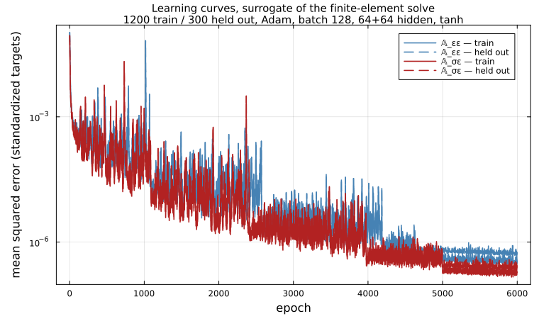

using MeanFieldHom
using TensND
using LinearAlgebra
using Printf
using Plots

gr()
default(; left_margin = 5Plots.mm, bottom_margin = 5Plots.mm)

const NI = MeanFieldHom.NeuralInclusions

MeanFieldHom.NeuralInclusions

§3 Using it

The same three lines as any other inclusion. The morphology parameters are passed as shape_params — they are the surrogate's features and the fields the sensitivity API differentiates — and the constituents as properties, which back both the contrast features and the Voigt/Reuss bounds.

ce(E, ν) = iso_stiffness(E / (3 * (1 - 2ν)), E / (2 * (1 + ν)))

const NU = 0.2
const E0 = 20.0                       # fresh cement paste, GPa
const C0 = ce(E0, NU)
const C1 = ce(3.5 * E0, NU)           # old natural aggregate

strain_s = load_surrogate(model_path("excentered_sphere_strain"))
stress_s = load_surrogate(model_path("excentered_sphere_stress"))

@printf(
    "surrogate of 𝔸_εε : %s, worst held-out error %.2e\n",
    join(NI.layer_widths(strain_s.net), "→"), worst_error(strain_s.provenance)
)
@printf(
    "surrogate of 𝔸_σε : %s, worst held-out error %.2e\n",
    join(NI.layer_widths(stress_s.net), "→"), worst_error(stress_s.provenance)
)

function nn_rca(α, w, e2)
    C2 = ce(e2 * E0, NU)
    return NeuralLocalizationInclusion(
        (1.0, 1.0, 1.0);
        strain = strain_s, stress = stress_s,
        shape_params = (; eccentricity = α, core_fraction = w),
        fractions = (w, 1 - w), properties = (C1, C2),
        guard = :error,
    )
end

println()
check_inclusion_interface(nn_rca(0.4, 0.5, 0.4))

true

§4 Against the finite elements

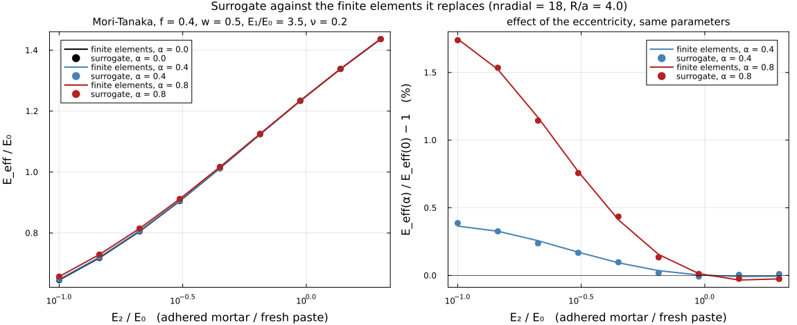
Committed, like everything measured against the teacher: a documentation build must not mesh anything. scripts/nn/make_excentered_figures.jl produces both the figure and the table below.

for f in ("excentered_report.md", "excentered_comparison.md")
    path = joinpath(NI.MODEL_DIR, f)
    isfile(path) && print(read(path, String), "\n")
end

<!-- Generated by scripts/nn/train_excentered.jl — do not edit by hand. -->

# Surrogate of the finite-element eccentric sphere

- teacher: `fe_axi_localization`, `nradial = 18`, `R/a = 4.0`
- one cold finite-element evaluation: **1.57 s**
- box: `α ∈ [0, 0.8]`, `w ∈ [0.2, 0.7]`, `E₂/E₀ ∈ [0.1, 2]`; fixed `ν = 0.2`, `E₁/E₀ = 3.5`
- 1200 training + 300 held-out solves

| surrogate | network | worst held-out error |
| --- | --- | ---: |
| `𝔸_εε` | 3→64→64→6 | 6.531e-04 |
| `𝔸_σε` | 3→64→64→6 | 6.802e-04 |

<!-- Generated by scripts/nn/make_excentered_figures.jl — do not edit by hand. -->

Mori-Tanaka, `f = 0.4`, `w = 0.5`, `E₁/E₀ = 3.5`, `ν = 0.2`,
`nradial = 18`, `R/a = 4.0`; `E₂/E₀` swept over a decade and a half.

| Quantity | Worst relative deviation from the finite elements |
| --- | ---: |
| `𝔸_εε` (the tensor itself) | 7.67e-04 |
| `E_eff/E₀` at α = 0.0 | 2.79e-04 |
| `E_eff/E₀` at α = 0.4 | 1.53e-04 |
| `E_eff/E₀` at α = 0.8 | 2.82e-04 |

| Cost of one evaluation | |
| --- | ---: |
| finite elements, cold | 0.868 s |
| surrogate | 3.4 µs |
| **speed-up** | **258444×** |

§5 In a scheme

Gate B with both tensors means the contributions take the exact heterogeneous branch, ℕ = 𝔸_σε − ℂ₀:𝔸_εε, and every scheme that consumes them works.

function rve_of(incl, f)
    r = RVE(:paste)
    add_matrix!(r, Ellipsoid(1.0), Dict(:C => C0))
    add_phase!(r, :rca, incl, Dict(:C => C0); fraction = f)
    return r
end

iso(C) = MeanFieldHom.Core.isotropify(C)

println("\n  Recycled-aggregate mortar, f = 0.4, w = 0.5, E₁/E₀ = 3.5, ν = 0.2")
println("  Mori-Tanaka, effective Young modulus E_eff/E₀\n")
@printf "  %8s %10s %10s %10s\n" "E₂/E₀" "α = 0" "α = 0.4" "α = 0.8"
for e2 in (0.1, 0.25, 0.5, 1.0, 2.0)
    vals = map((0.0, 0.4, 0.8)) do α
        C = homogenize(rve_of(nn_rca(α, 0.5, e2), 0.4), MoriTanaka(), :C)
        k, μ = k_mu(iso(C))
        9k * μ / (3k + μ) / E0
    end
    @printf "  %8.2f %10.4f %10.4f %10.4f\n" e2 vals...
end

  Recycled-aggregate mortar, f = 0.4, w = 0.5, E₁/E₀ = 3.5, ν = 0.2
  Mori-Tanaka, effective Young modulus E_eff/E₀

     E₂/E₀      α = 0    α = 0.4    α = 0.8
      0.10     0.6456     0.6481     0.6569
      0.25     0.8484     0.8503     0.8569
      0.50     1.0458     1.0465     1.0492
      1.00     1.2499     1.2497     1.2500
      2.00     1.4365     1.4366     1.4361

The eccentricity stiffens the composite while the shell is the weak phase — the eccentric pattern short-circuits part of the soft mortar — and the effect changes sign once the shell is stiffer than the paste. That is the physical content of the finite-element study, reproduced here at microsecond cost.

§6 The gain

Two numbers, measured on this machine. The finite-element figure is the cold one, since an iterative scheme changes its reference medium at every iteration and never hits the cache.

const N_EVAL = 2000
incl = nn_rca(0.4, 0.5, 0.4)
strain_strain_loc(incl, C0, C0)                  # warm up the compilation
t_nn = @elapsed for _ in 1:N_EVAL
    strain_strain_loc(incl, C0, C0)
end

@printf(
    "\n  %d surrogate evaluations : %.3f s  (%.1f µs each)\n",
    N_EVAL, t_nn, 1.0e6t_nn / N_EVAL
)
println("  the finite-element figure it replaces is in the table of §4.")

  2000 surrogate evaluations : 0.008 s  (4.0 µs each)
  the finite-element figure it replaces is in the table of §4.

§7 What the finite elements cannot do

The surrogate is smooth in its inputs, so ForwardDiff reaches the eccentricity — a morphology parameter — straight through the scheme. MeanFieldHom.FiniteElements refuses the same request outright, and rightly: its solve would silently return zero.

idx = C -> get_array(C)[1, 1, 1, 1]

println("\n  ∂C₁₁₁₁/∂α through a Mori-Tanaka estimate, f = 0.4, w = 0.5, E₂/E₀ = 0.4")
println("  ", "-"^58)
@printf "  %8s %16s %16s\n" "α" "AD" "finite differences"
for α in (0.1, 0.3, 0.5, 0.7)
    d = derivative(
        rve_of(nn_rca(α, 0.5, 0.4), 0.4), MoriTanaka(),
        geometry(:rca, :shape_params, 1); indexer = idx
    )
    h = 1.0e-5
    fd = (
        idx(homogenize(rve_of(nn_rca(α + h, 0.5, 0.4), 0.4), MoriTanaka())) -
            idx(homogenize(rve_of(nn_rca(α - h, 0.5, 0.4), 0.4), MoriTanaka()))
    ) / (2h)
    @printf "  %8.2f %16.6f %16.6f\n" α d fd
end

  ∂C₁₁₁₁/∂α through a Mori-Tanaka estimate, f = 0.4, w = 0.5, E₂/E₀ = 0.4
  ----------------------------------------------------------
         α               AD finite differences
      0.10         0.022168         0.022168
      0.30         0.076721         0.076721
      0.50         0.184402         0.184402
      0.70         0.277614         0.277614

The two columns agree, and neither is zero: the sensitivity of the effective stiffness to how far off centre the old aggregate sits is now a quantity one can compute — and optimize against.

This page was generated using Literate.jl.