Carbonation of a Cement Paste

Before this page

CO₂ Dissolution and the Carbonate System and Effect of Water/Cement Ratio on Cement Hydration.

Carbonation is the principal durability threat to reinforced concrete. Atmospheric CO₂ diffuses into the concrete cover, dissolves into the pore water, and reacts with the alkaline hydration products — above all portlandite Ca(OH)₂ and calcium silicate hydrates (CSH) — to precipitate calcium carbonate (calcite):

This consumption of alkalinity drives the pore-solution pH from ≈ 12.5–13 down to ≈ 8–9, below the passivation threshold of the steel reinforcement (~9.5). The depth at which pH drops below this threshold is the carbonation front.

This example simulates the progressive carbonation of a reference hydrated cement paste by scanning the CO₂ intake from zero to 2.5× the stoichiometric portlandite capacity. It tracks the pH of the pore solution, the depletion of portlandite and CSH, and the accumulation of calcite.

System setup

The CEMDATA18-merged database is used here because it contains both the cement hydration products and the carbonate mineral phases (calcite Cal, monocarbonate, hemicarbonate) within a single consistent dataset.

The species list covers the full mineralogy of a hydrating and carbonating Portland cement paste: clinker phases, classic hydration products, and the three principal carbonation products.

Group	Symbols	Role
Clinker	`C3S C2S C3A C4AF Gp`	Initial anhydrous phases
Hydration products	`Portlandite Jennite ettringite monosulphate12 C3AH6`	Formed during hydration
Carbonation products	`Cal monocarbonate hemicarbonate`	Formed on CO₂ uptake
CO₂ input	`CO2@`	Dissolved CO₂ entering the pore solution

julia

input_species = split("""C3S C2S C3A C4AF Gp
                         Portlandite Jennite ettringite monosulphate12 C3AH6
                         Cal monocarbonate hemicarbonate
                         CO2@""")

species = speciation(
    substances, input_species;
    aggregate_state   = [AS_AQUEOUS],
    exclude_species   = split("H2@ O2@ H2S@ HS- thaumasite Arg"),
    include_species   = input_species,
)

cs = ChemicalSystem(species, CEMDATA_PRIMARIES)

The chemical system in full — species, phases and the conservation matrix

julia

cs

58-element ChemicalSystem{Species, AbstractReaction, StoichMatrix{Real, Symbol, Vector{Symbol}, Matrix{Real}, Species}, StoichMatrix{Real, Species, Vector{Species}, Matrix{Real}, Species}, Nothing, Nothing}:
 H2O@ {H2O  l} [H2O@ ◆ H₂O@]
 CaSiO3@ {CaSiO3  aq } [CaSiO3@ ◆ CaSiO₃@]
 SiO3-2 {SiO3-2  aq } [SiO3-2 ◆ SiO₃²⁻]
 AlSiO5-3 {AlSiO5-3  aq } [AlSiO5-3 ◆ AlSiO₅³⁻]
 Si4O10-4 {Si4O10-4  aq } [Si4O10-4 ◆ Si₄O₁₀⁴⁻]
 SiO2@ {SiO2  aq ( + 2 H2O = Si(OH)4  aq )} [SiO2@ ◆ SiO₂@]
 Al(SO4)2- {Al(SO4)2-} [Al(SO4)2- ◆ Al(SO₄)₂⁻]
 Fe(SO4)@ {FeSO4  aq} [Fe(SO4)@ ◆ Fe(SO₄)@]
 Fe(SO4)+ {FeSO4+} [Fe|3|(SO4)+ ◆ Fe(SO₄)⁺]
 Fe(SO4)2- {Fe(SO4)2-} [Fe|3|(SO4)2- ◆ Fe(SO₄)₂⁻]
 Fe(CO3)@ {FeCO3  aq} [FeCO3@ ◆ FeCO₃@]
 Al(SO4)+ {AlSO4+} [Al(SO4)+ ◆ Al(SO₄)⁺]
 Fe(HCO3)+ {FeHCO3+} [FeHCO3+ ◆ FeHCO₃⁺]
 Fe(HSO4)+2 {FeHSO4+2} [Fe|3|HSO4+2 ◆ FeHSO₄²⁺]
 Fe(HSO4)+ {FeHSO4+} [FeHSO4+ ◆ FeHSO₄⁺]
 Al+3 {Al+3} [Al+3 ◆ Al³⁺]
 Ca+2 {Ca+2} [Ca+2 ◆ Ca²⁺]
 Fe+2 {Fe+2} [Fe+2 ◆ Fe²⁺]
 H+ {H+} [H+ ◆ H⁺]
 HCO3- {HCO3-} [HCO3- ◆ HCO₃⁻]
 SO4-2 {SO4-2} [S|6|O4-2 ◆ SO₄²⁻]
 AlO2- {AlO2-  ( + 2 H2O = Al(OH)4- )} [AlO2- ◆ AlO₂⁻]
 CO3-2 {CO3-2} [CO3-2 ◆ CO₃²⁻]
 FeO2- {FeO2- ( + 2 H2O = Fe(OH)4- )} [Fe|3|O2- ◆ FeO₂⁻]
 AlOH+2 {AlOH+2} [Al(OH)+2 ◆ Al(OH)²⁺]
 AlO+ {AlO+  ( + H2O = Al(OH)2+ )} [AlO+ ◆ AlO⁺]
 AlO2H@ {AlO2H  aq ( + 2H2O = Al(OH)3  aq )} [AlO2H@ ◆ AlO₂H@]
 CaOH+ {CaOH+} [Ca(OH)+ ◆ Ca(OH)⁺]
 FeOH+2 {FeOH+2} [Fe|3|(OH)+2 ◆ Fe(OH)²⁺]
 FeO+ {FeO+ ( + H2O = Fe(OH)2+ )} [Fe|3|O+ ◆ FeO⁺]
 FeO2H@ {FeO2H  aq  ( + H2O = Fe(OH)3  aq)} [Fe|3|O2H@ ◆ FeO₂H@]
 FeOH+ {FeOH+} [FeOH+ ◆ FeOH⁺]
 HSO3- {HSO3-} [HS|4|O3- ◆ HSO₃⁻]
 HSO4- {HSO4-} [HS|6|O4- ◆ HSO₄⁻]
 OH- {OH-} [OH- ◆ OH⁻]
 S2O3-2 {S2O3-2} [S|2|2O3-2 ◆ S₂O₃²⁻]
 SO3-2 {SO3-2} [S|4|O3-2 ◆ SO₃²⁻]
 Fe+3 {Fe+3} [Fe|3|+3 ◆ Fe³⁺]
 CH4@ {CH4  aq} [C|-4|H4@ ◆ CH₄@]
 Ca(HCO3)+ {CaHCO3+} [Ca(HCO3)+ ◆ Ca(HCO₃)⁺]
 Ca(HSiO3)+ {CaHSiO3+  ( + H2O = CaSiO(OH)3+ )} [Ca(HSiO3)+ ◆ Ca(HSiO₃)⁺]
 CO2@ {CO2  aq} [CO2@ ◆ CO₂@]
 Ca(CO3)@ {CaCO3  aq} [CaCO3@ ◆ CaCO₃@]
 Ca(SO4)@ {CaSO4  aq} [CaSO4@ ◆ CaSO₄@]
 HSiO3- {HSiO3-  ( + H2O = SiO(OH)3- )} [HSiO3- ◆ HSiO₃⁻]
 monosulphate12 {Monosulphate12} [Ca4Al2SO10(H2O)12 ◆ Ca₄Al₂SO₁₀(H₂O)₁₂]
 Jennite {Jennite   10/6 end-member of  id CSH SS (norm per 1 Si)  } [(SiO2)1(CaO)1.666667(H2O)2.1 ◆ (SiO₂)₁(CaO)₅//₃(H₂O)₂.₁]
 monocarbonate {Monocarbonate} [Ca4Al2CO9(H2O)11 ◆ Ca₄Al₂CO₉(H₂O)₁₁]
 C3S {C3S} [(CaO)3SiO2 ◆ (CaO)₃SiO₂]
 C2S {C2S-beta} [(CaO)2SiO2 ◆ (CaO)₂SiO₂]
 C3A {C3A (3CaO_Al2O3)} [(CaO)3Al2O3 ◆ (CaO)₃Al₂O₃]
 C4AF {C4AF} [(CaO)4(Al2O3)(Fe|3|2O3) ◆ (CaO)₄(Al₂O₃)(Fe₂O₃)]
 ettringite {Ettringite with 32 H2O} [((H2O)2)Ca6Al2(SO4)3(OH)12(H2O)24 ◆ ((H₂O)₂)Ca₆Al₂(SO₄)₃(OH)₁₂(H₂O)₂₄]
 C3AH6 {C3AH6} [Ca3Al2O6(H2O)6 ◆ Ca₃Al₂O₆(H₂O)₆]
 hemicarbonate {Hemicarbonate} [(CaO)3Al2O3(CaCO3)0.5(CaO2H2)0.5(H2O)11.5 ◆ (CaO)₃Al₂O₃(CaCO₃)½(CaO₂H₂)½(H₂O)₂₃//₂]
 Portlandite {Portlandite} [Ca(OH)2 ◆ Ca(OH)₂]
 Gp {Gypsum} [CaSO4(H2O)2 ◆ CaSO₄(H₂O)₂]
 Cal {Calcite} [CaCO3 ◆ CaCO₃]

Why cemdata18-merged?

Not for calcite: Cal is present in cemdata18-thermofun.json too, and an earlier version of this note said otherwise. Nor for species at all — both files describe the same 228 substances. What the PHREEQC .dat file brings is the reactions, 148 against 7, and with them the phase-volume data that makes volumes and porosity available on one consistent dataset.

Building the equilibrium solver

A single solver is compiled once and reused for all calculations.

julia

using Optimization, OptimizationIpopt

opt = IpoptOptimizer(
    acceptable_tol        = 1e-10,
    dual_inf_tol          = 1e-10,
    acceptable_iter       = 100,
    constr_viol_tol       = 1e-10,
    warm_start_init_point = "no",
)

solver = EquilibriumSolver(
    cs,
    DiluteSolutionModel(),
    opt;
    variable_space = Val(:linear),
    abstol  = 1e-8,
    reltol  = 1e-8,
)

sp_idx = Dict(symbol(s) => i for (i, s) in enumerate(cs.species))

Dict{String, Int64} with 58 entries:
  "SiO2@"          => 6
  "AlO2-"          => 22
  "Fe(HCO3)+"      => 13
  "Fe(CO3)@"       => 11
  "Fe(SO4)@"       => 8
  "FeO2-"          => 24
  "HSiO3-"         => 45
  "C3AH6"          => 54
  "S2O3-2"         => 36
  "FeO+"           => 30
  "Fe+2"           => 18
  "FeOH+2"         => 29
  "SO4-2"          => 21
  "Jennite"        => 47
  "Si4O10-4"       => 5
  "Al(SO4)2-"      => 7
  "monocarbonate"  => 48
  "CO2@"           => 42
  "Fe(SO4)+"       => 9
  "C3S"            => 49
  "CaSiO3@"        => 2
  "CO3-2"          => 23
  "Al+3"           => 16
  "Cal"            => 58
  "Fe(HSO4)+2"     => 14
  "Ca+2"           => 17
  "HSO4-"          => 34
  "HSO3-"          => 33
  "OH-"            => 35
  "AlOH+2"         => 25
  "H2O@"           => 1
  "Ca(HCO3)+"      => 40
  "C3A"            => 51
  "Al(SO4)+"       => 12
  "FeOH+"          => 32
  "C4AF"           => 52
  "hemicarbonate"  => 55
  "FeO2H@"         => 31
  "SO3-2"          => 37
  "SiO3-2"         => 3
  "CaOH+"          => 28
  "AlSiO5-3"       => 4
  "HCO3-"          => 20
  "H+"             => 19
  "Fe+3"           => 38
  "CH4@"           => 39
  "Fe(SO4)2-"      => 10
  "monosulphate12" => 46
  "ettringite"     => 53
  "Ca(CO3)@"       => 43
  "Gp"             => 57
  "AlO2H@"         => 27
  "Portlandite"    => 56
  "Ca(HSiO3)+"     => 41
  "Ca(SO4)@"       => 44
  "AlO+"           => 26
  "C2S"            => 50
  "Fe(HSO4)+"      => 15

Step 1 — Reference hydrated paste (no CO₂)

Before scanning the carbonation, the reference state of the fully hydrated paste is established by solving the equilibrium without any CO₂ input. This gives the initial portlandite inventory, which is used to normalize the CO₂ axis.

julia

compo = ["C3S" => 0.678, "C2S" => 0.166, "C3A" => 0.040, "C4AF" => 0.072, "Gp" => 0.028]
c     = sum(last.(compo))   # ≈ 0.984
wc    = 0.40
w     = wc * c
mtot  = c + w

state0 = ChemicalState(cs)
for (sym, mfrac) in compo
    set_quantity!(state0, sym, mfrac / mtot * u"kg")
end
set_quantity!(state0, "H2O@", w / mtot * u"kg")

V0 = volume(state0)
set_quantity!(state0, "H+",  1e-7u"mol/L" * V0.liquid)
set_quantity!(state0, "OH-", 1e-7u"mol/L" * V0.liquid)

ref = solve(solver, state0)

n_port0 = ustrip(ref.n[sp_idx["Portlandite"]])
n_ett0  = ustrip(ref.n[sp_idx["ettringite"]])
n_jen0  = ustrip(ref.n[sp_idx["Jennite"]])

println("Reference state (w/c = 0.40, no CO₂):")
println("  pH          = ", round(pH(ref),         digits = 2))
println("  Portlandite = ", round(n_port0,          digits = 3), " mol/kg")
println("  Ettringite  = ", round(n_ett0,           digits = 3), " mol/kg")
println("  Jennite     = ", round(n_jen0,           digits = 3), " mol/kg")
println("  Porosity    = ", round(porosity(ref)*100), " %")

┌ Warning: Verbosity toggle: missing_second_order_ad
│  The selected optimization algorithm requires second order derivatives, but `SecondOrder` ADtype was not provided. So a `SecondOrder` with AutoForwardDiff() for both inner and outer will be created, this can be suboptimal and not work in some cases so an explicit `SecondOrder` ADtype is recommended.
└ @ OptimizationBase ~/.julia/packages/OptimizationBase/BEgWO/src/cache.jl:116
┌ Info: Verbosity toggle: unsupported_kwargs
└  common abstol is currently not used by IpoptOptimizer(1.0e-10, 100, 1.0e-10, 1.0e-10, 0.0001, "no", "no", "mumps", "none", "", "", "yes", "gradient-based", 100.0, "no", "no", "monotone", "quality-function", 0.1, "obj-constr-filter", "no", "exact", 6, "bfgs", "no", "filter", "no", Dict{String, Any}())
This is Ipopt version 3.14.19, running with linear solver MUMPS 5.9.0.

Number of nonzeros in equality constraint Jacobian...:      522
Number of nonzeros in inequality constraint Jacobian.:        0
Number of nonzeros in Lagrangian Hessian.............:     1711

Total number of variables............................:       58
                     variables with only lower bounds:        0
                variables with lower and upper bounds:       58
                     variables with only upper bounds:        0
Total number of equality constraints.................:        9
Total number of inequality constraints...............:        0
        inequality constraints with only lower bounds:        0
   inequality constraints with lower and upper bounds:        0
        inequality constraints with only upper bounds:        0

iter    objective    inf_pr   inf_du lg(mu)  ||d||  lg(rg) alpha_du alpha_pr  ls
   0 -5.3323690e+03 5.83e-01 6.84e-01  -1.0 0.00e+00    -  0.00e+00 0.00e+00   0
   1 -5.2805107e+03 4.97e-01 3.02e+00  -1.0 1.37e+00    -  3.24e-01 1.47e-01f  1
   2 -5.1968367e+03 3.35e-01 4.36e+00  -1.0 4.50e+00    -  2.60e-01 3.26e-01f  1
   3 -5.1780328e+03 3.04e-01 1.43e+01  -1.0 3.59e+00    -  3.94e-01 9.24e-02h  1
   4 -5.0890866e+03 1.27e-01 1.96e+01  -1.0 2.82e+00    -  8.24e-01 5.82e-01h  1
   5 -5.0568212e+03 5.91e-02 5.54e+01  -1.0 3.83e+00    -  8.39e-01 5.35e-01h  1
   6 -5.0359262e+03 2.82e-02 1.87e+02  -1.0 1.51e+00    -  9.98e-01 5.24e-01h  1
   7 -5.0234836e+03 1.02e-02 3.28e+02  -1.0 6.33e-01    -  1.00e+00 6.39e-01h  1
   8 -5.0197150e+03 4.82e-03 1.09e+03  -1.0 1.59e-01    -  1.00e+00 5.26e-01h  1
   9 -5.0175124e+03 1.70e-03 1.87e+03  -1.0 7.43e-02    -  1.00e+00 6.47e-01h  1
iter    objective    inf_pr   inf_du lg(mu)  ||d||  lg(rg) alpha_du alpha_pr  ls
  10 -5.0168870e+03 8.16e-04 6.59e+03  -1.0 2.61e-02    -  1.00e+00 5.20e-01h  1
  11 -5.0165118e+03 2.86e-04 1.10e+04  -1.0 1.26e-02    -  1.00e+00 6.49e-01h  1
  12 -5.0164066e+03 1.38e-04 3.92e+04  -1.0 4.40e-03    -  1.00e+00 5.19e-01h  1
  13 -5.0163432e+03 4.82e-05 6.52e+04  -1.0 2.12e-03    -  1.00e+00 6.49e-01h  1
  14 -5.0163421e+03 4.67e-05 4.68e+05  -1.0 7.41e-04    -  1.00e+00 3.24e-02f  5
  15 -5.0163178e+03 1.25e-05 2.41e+05  -1.0 7.17e-04    -  1.00e+00 7.32e-01h  1
  16 -5.0163123e+03 4.67e-06 6.94e+05  -1.0 1.92e-04    -  1.00e+00 6.26e-01h  1
  17 -5.0163122e+03 4.52e-06 4.84e+06  -1.0 7.17e-05    -  1.00e+00 3.26e-02f  5
  18 -5.0163098e+03 1.20e-06 2.48e+06  -1.0 6.94e-05    -  1.00e+00 7.33e-01h  1
  19 -5.0163093e+03 4.48e-07 7.11e+06  -1.0 1.85e-05    -  1.00e+00 6.28e-01h  1
iter    objective    inf_pr   inf_du lg(mu)  ||d||  lg(rg) alpha_du alpha_pr  ls
  20 -5.0163093e+03 4.33e-07 4.96e+07  -1.0 6.88e-06    -  1.00e+00 3.28e-02f  5
  21 -5.0163090e+03 1.13e-07 2.47e+07  -1.0 6.65e-06    -  1.00e+00 7.39e-01h  1
  22 -5.0163090e+03 3.99e-08 6.68e+07  -1.0 1.74e-06    -  1.00e+00 6.46e-01h  1
  23 -5.0163090e+03 3.71e-08 4.39e+08  -1.0 6.13e-07    -  1.00e+00 7.02e-02f  4
  24 -5.0163090e+03 7.29e-09 1.60e+08  -1.0 5.70e-07    -  1.00e+00 8.04e-01h  1
  25 -5.0163090e+03 6.89e-09 1.16e+09  -1.0 1.12e-07    -  1.00e+00 5.43e-02f  5
  26 -5.0163090e+03 3.55e-15 2.04e-01  -1.0 1.06e-07    -  1.00e+00 1.00e+00h  1
  27 -5.0435855e+03 1.78e-15 1.11e+09  -8.6 1.18e+00    -  5.97e-01 1.00e+00f  1
  28 -5.0641089e+03 3.55e-15 3.96e+08  -8.6 3.49e+00    -  6.42e-01 7.48e-01f  1
  29 -5.0769011e+03 3.55e-15 1.95e+08  -8.6 8.27e-01    -  5.07e-01 8.97e-01f  1
iter    objective    inf_pr   inf_du lg(mu)  ||d||  lg(rg) alpha_du alpha_pr  ls
  30 -5.0787902e+03 1.78e-15 8.90e+07  -8.6 2.06e-01    -  5.44e-01 6.02e-01f  1
  31 -5.0815638e+03 3.55e-15 7.92e+07  -8.6 3.18e-01    -  1.10e-01 9.15e-01f  1
  32 -5.0819083e+03 5.55e-17 3.73e+07  -8.6 1.60e-02    -  5.30e-01 9.67e-01f  1
  33 -5.0819619e+03 3.55e-15 2.46e+07  -8.6 5.78e-03    -  3.41e-01 9.99e-01f  1
  34 -5.0819702e+03 4.44e-16 4.65e+05  -8.6 1.98e-03    -  9.81e-01 1.00e+00f  1
  35 -5.0819727e+03 3.55e-15 3.36e+05  -8.6 1.32e-03    -  2.79e-01 1.00e+00f  1
  36 -5.0819729e+03 3.55e-15 1.47e-02  -8.6 2.80e-04    -  1.00e+00 1.00e+00f  1
  37 -5.0819730e+03 3.55e-15 2.01e-02  -8.6 1.65e-04    -  7.59e-01 1.00e+00f  1
  38 -5.0819730e+03 3.55e-15 5.33e-03  -8.6 2.70e-05    -  1.00e+00 1.00e+00h  1
  39 -5.0819730e+03 3.55e-15 4.17e-03  -8.6 2.62e-06    -  1.00e+00 1.00e+00h  1
iter    objective    inf_pr   inf_du lg(mu)  ||d||  lg(rg) alpha_du alpha_pr  ls
  40 -5.0819730e+03 3.55e-15 8.43e-04  -8.6 2.23e-07    -  1.00e+00 1.00e+00h  1
  41 -5.0819730e+03 3.55e-15 4.20e-05  -8.6 1.56e-08    -  1.00e+00 1.00e+00h  1
  42 -5.0819730e+03 3.55e-15 6.82e-08  -8.6 4.10e-10    -  1.00e+00 1.00e+00h  1
  43 -5.0819730e+03 3.55e-15 2.13e-13  -8.6 6.27e-13    -  1.00e+00 1.00e+00h  1

Number of Iterations....: 43

                                   (scaled)                 (unscaled)
Objective...............:  -8.2849175945089073e+01   -5.0819730212598924e+03
Dual infeasibility......:   2.1330779044305405e-13    1.3084311628816093e-11
Constraint violation....:   3.5527136788005009e-15    3.5527136788005009e-15
Variable bound violation:   7.1112780026506333e-11    7.1112780026506333e-11
Complementarity.........:   2.5059035597733371e-09    1.5371226254667529e-07
Overall NLP error.......:   2.5059035597733371e-09    1.5371226254667529e-07


Number of objective function evaluations             = 63
Number of objective gradient evaluations             = 44
Number of equality constraint evaluations            = 63
Number of inequality constraint evaluations          = 0
Number of equality constraint Jacobian evaluations   = 44
Number of inequality constraint Jacobian evaluations = 0
Number of Lagrangian Hessian evaluations             = 43
Total seconds in IPOPT                               = 7.887

EXIT: Optimal Solution Found.
Reference state (w/c = 0.40, no CO₂):
  pH          = 11.33
  Portlandite = 3.106 mol/kg
  Ettringite  = 0.0 mol/kg
  Jennite     = 2.855 mol/kg
  Porosity    = 19.0 %

Step 2 — Progressive CO₂ uptake

For each CO₂ level, the clinker phases and water are set as in the reference state and an additional amount of CO2@ is added. The solver finds the equilibrium that minimizes the total Gibbs free energy, distributing CO₂ between the dissolved carbonate species, calcite and the AFm carbonate phases while consuming portlandite and, at higher dosages, CSH.

The CO₂ axis is normalized by n_port0 so that ξ = n(CO₂)/n(Portlandite)₀. Full carbonation of portlandite alone corresponds to ξ = 1.

julia

ξ_range = range(0, 2.5; length = 50)   # dimensionless CO₂ / portlandite ratio

pH_vals      = Float64[]
n_Port_vals  = Float64[]
n_Cal_vals   = Float64[]
n_Monoc_vals = Float64[]
n_Jen_vals   = Float64[]

state = ChemicalState(cs)

for ξ in ξ_range
    n_CO2 = ξ * n_port0   # mol of CO₂ added per kg total paste

    for (sym, mfrac) in compo
        set_quantity!(state, sym, mfrac / mtot * u"kg")
    end
    set_quantity!(state, "H2O@",  w / mtot   * u"kg")
    set_quantity!(state, "CO2@",  n_CO2      * u"mol")

    V = volume(state)
    set_quantity!(state, "H+",  1e-7u"mol/L" * V.liquid)
    set_quantity!(state, "OH-", 1e-7u"mol/L" * V.liquid)

    state_eq = solve(solver, state)

    push!(pH_vals,      pH(state_eq))
    push!(n_Port_vals,  ustrip(state_eq.n[sp_idx["Portlandite"]]))
    push!(n_Cal_vals,   ustrip(state_eq.n[sp_idx["Cal"]]))
    push!(n_Monoc_vals, ustrip(state_eq.n[sp_idx["monocarbonate"]]))
    push!(n_Jen_vals,   ustrip(state_eq.n[sp_idx["Jennite"]]))
end

Results

pH of the pore solution

julia

using Plots

p1 = plot(
    collect(ξ_range), pH_vals;
    xlabel     = "CO₂ / Portlandite₀  (mol/mol)",
    ylabel     = "Pore solution pH",
    label      = "Numerical (ChemistryLab)",
    linewidth  = 2,
    marker     = :circle,
    markersize = 4,
    color      = :steelblue,
    title      = "pH during carbonation (w/c = 0.40)",
    ylims      = (7, 14),
    legend     = :topright,
)
hline!(p1, [9.5];  linestyle = :dash, color = :red,
       label = "Depassivation threshold (pH 9.5)")
hline!(p1, [pH(ref)]; linestyle = :dot, color = :grey,
       label = "Initial pH")
vline!(p1, [1.0];  linestyle = :dot, color = :orange,
       label = "ξ = 1 (portlandite stoichiometry)")
p1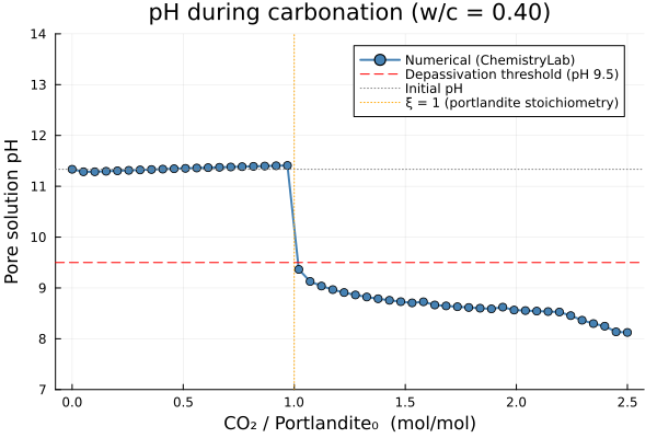

Phase evolution

julia

p2 = plot(
    collect(ξ_range), n_Port_vals ./ n_port0;
    xlabel     = "CO₂ / Portlandite₀  (mol/mol)",
    ylabel     = "Relative amount  (–)",
    label      = "Portlandite  Ca(OH)₂",
    linewidth  = 2,
    marker     = :circle,
    markersize = 4,
    color      = :steelblue,
    title      = "Phase assemblage during carbonation",
    ylims      = (0, 1.05),
    legend     = :topright,
)
plot!(p2, collect(ξ_range), n_Cal_vals   ./ n_port0;
    label     = "Calcite  CaCO₃",
    linewidth = 2, marker = :square, markersize = 4, color = :firebrick,
)
plot!(p2, collect(ξ_range), n_Monoc_vals ./ n_port0;
    label     = "Monocarbonate",
    linewidth = 2, marker = :diamond, markersize = 4, color = :orange,
)
plot!(p2, collect(ξ_range), n_Jen_vals   ./ n_jen0;
    label     = "Jennite (CSH)  – rescaled",
    linewidth = 2, marker = :utriangle, markersize = 4, color = :green,
    linestyle = :dash,
)
vline!(p2, [1.0]; linestyle = :dot, color = :grey, label = "ξ = 1")
p2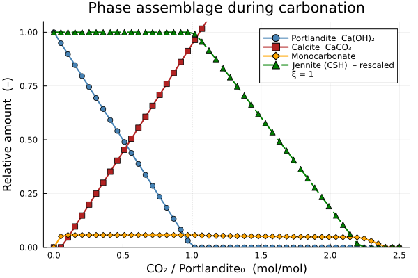

Analysis

The simulation reveals four successive zones as CO₂ uptake increases:

Zone	ξ range	Dominant reaction	pH
I — AFm conversion	0 → ~0.2	monosulphate + CO₂ → monocarbonate + gypsum	≈ 12.5
II — Portlandite buffering	~0.2 → 1	Portlandite + CO₂ → calcite + H₂O	≈ 12.0–12.5
III — Portlandite depletion	ξ ≈ 1	Portlandite exhausted; pH drops sharply	12 → 9.5
IV — CSH decalcification	1 → 2.5	Jennite (CSH) + CO₂ → calcite + amorphous SiO₂·xH₂O	9–10

Key observations:

Zone I: CO₂ first attacks the monosulphate and ettringite, converting them to monocarbonate. pH remains nearly constant because portlandite acts as a reservoir.
Zone II: Once the AFm phases are saturated, portlandite is consumed 1:1 by CO₂ to form calcite. The high solubility of portlandite maintains pH ≈ 12–12.5.
Zone III: The depletion of portlandite at ξ ≈ 1 triggers a sharp pH drop, crossing the steel passivation threshold (9.5). This is the thermodynamic equivalent of the carbonation front passing through the concrete cover.
Zone IV: Above ξ = 1, CSH (Jennite) is decalcified; pH stabilizes around 9–10 before eventually reaching the CO₂/HCO₃⁻ equilibrium (~8.3).

From equilibrium to service life

ChemistryLab provides the thermodynamic driving forces at each CO₂ exposure level. To translate this into a carbonation depth as a function of time, couple the phase diagram above with a diffusion model: the front advances when the local CO₂ concentration exceeds the buffering capacity per unit volume of paste, which is directly read from the ξ-axis at the portlandite depletion point.

Link to the carbonate system

The aqueous speciation within the carbonating pore solution — distribution between CO₂(aq), HCO₃⁻ and CO₃²⁻ — follows the same equilibria described in the CO₂ dissolution example. In the high-pH pore solution (pH > 12), CO₃²⁻ dominates; below pH 8.3, CO₂(aq) takes over.

Where to go next

The binders that replace part of the clinker, and change what there is to carbonate, are mapped in The binders, and what distinguishes them and computed from Two CEM II onwards.

Carbonation of a Cement Paste ​

System setup ​

Building the equilibrium solver ​

Step 1 — Reference hydrated paste (no CO₂) ​

Step 2 — Progressive CO₂ uptake ​

Results ​

pH of the pore solution ​

Phase evolution ​

Analysis ​

Where to go next ​

Carbonation of a Cement Paste

System setup

Building the equilibrium solver

Step 1 — Reference hydrated paste (no CO₂)

Step 2 — Progressive CO₂ uptake

Results

pH of the pore solution

Phase evolution

Analysis

Where to go next