
The Pitzer model, and what it can be used with
Before this page
Activity models §6.
Activity models §6 derives the ion-interaction model and says why its Gibbs-Duhem consistency is exact rather than approximate. This page loads the shipped parameter set, checks that claim, and establishes what the set may and may not be combined with — which turns out to be the practical question.
using ChemistryLab
using DynamicQuantities
using ForwardDiff
using LinearAlgebra
using Printf

pars = build_pitzer_parameters(datapath("pitzer-reardon1990.toml"))
model = PitzerActivityModel(; parameters = pars)

substances = build_species(datapath("slop98-inorganic-thermofun.json"); verbose = false)
dict = Dict(symbol(s) => s for s in substances)
nacl = ChemicalSystem([dict[s] for s in split("H2O@ Na+ Cl-")], ["H2O@", "Na+", "Cl-"])
# the molar mass the closures themselves use, so a molality formed here is the
# one they form
M_w = ustrip(us"kg/mol", nacl.species[only(nacl.idx_solvent)][:M])
n_w = 1 / M_w
prm(k) = (ΔₐG⁰overRT = zeros(k), T = 298.15, P = 1.0e5, ϵ = 1.0e-30)
┌──────────────────────────────────────────────────────────┐
│ Loading database: data/slop98-inorganic-thermofun.json │
└──────────────────────────────────────────────────────────┘
┌────────────────────┐
│ Building species │
└────────────────────┘
Progress: 14%|██████████████████████ | ETA: 0:00:01[K
Progress: 27%|███████████████████████████████████████████▉ | ETA: 0:00:01[K
Progress: 41%|█████████████████████████████████████████████████████████████████▉ | ETA: 0:00:00[K
Progress: 54%|███████████████████████████████████████████████████████████████████████████████████████▋ | ETA: 0:00:00[K
Progress: 68%|█████████████████████████████████████████████████████████████████████████████████████████████████████████████▍ | ETA: 0:00:00[K
Progress: 81%|██████████████████████████████████████████████████████████████████████████████████████████████████████████████████████████████████▋ | ETA: 0:00:00[K
Progress: 89%|███████████████████████████████████████████████████████████████████████████████████████████████████████████████████████████████████████████████▌ | ETA: 0:00:00[K
Progress: 92%|████████████████████████████████████████████████████████████████████████████████████████████████████████████████████████████████████████████████████▏ | ETA: 0:00:00[K
Progress: 95%|████████████████████████████████████████████████████████████████████████████████████████████████████████████████████████████████████████████████████████▎ | ETA: 0:00:00[K
Progress: 98%|█████████████████████████████████████████████████████████████████████████████████████████████████████████████████████████████████████████████████████████████▌ | ETA: 0:00:00[K
Progress: 100%|█████████████████████████████████████████████████████████████████████████████████████████████████████████████████████████████████████████████████████████████████| Time: 0:00:01[K1. The set says which of its numbers were measured
Reardon's tables are those of Harvie, Møller and Weare, except that the silicate, aluminate and ferrate parameters had no published data at all and were estimated by analogy — he names the analog in each case. Those are exactly the ions a cement assemblage needs, so the set carries the distinction and pitzer_origin reads it back:
for (c, a) in (("Na+", "Cl-"), ("Ca+2", "SO4-2"), ("Ca+2", "OH-"),
               ("Ca+2", "Al(OH)4-"), ("Na+", "H3SiO4-"), ("Na+", "H2SiO4-2"))
    @printf("  %-5s / %-9s  β⁰ = %+8.4f   β¹ = %+8.4f   β² = %+8.2f   %s\n",
            c, a, pars.beta0[(c, a)], pars.beta1[(c, a)], pars.beta2[(c, a)],
            pitzer_origin(pars, c, a))
end
Na+ / Cl- β⁰ = +0.0765 β¹ = +0.2664 β² = +0.00 fitted
Ca+2 / SO4-2 β⁰ = +0.2000 β¹ = +3.1973 β² = -54.24 fitted
Ca+2 / OH- β⁰ = -0.1747 β¹ = -0.2303 β² = -5.72 fitted
Ca+2 / Al(OH)4- β⁰ = +0.2145 β¹ = +2.5300 β² = +0.00 estimated:HSO4-
Na+ / H3SiO4- β⁰ = +0.0454 β¹ = +0.3980 β² = +0.00 estimated:HSO4-
Na+ / H2SiO4-2 β⁰ = +0.0196 β¹ = +1.1130 β² = +0.00 estimated:SO4-2A β² appears only where the pair needs a third ionic-strength dependence — 2-2 electrolytes, and Ca–OH, which Harvie et al. treat the same way.
2. Against measurement, over four decades of molality
Internal consistency cannot tell a correct parameter set from a self-consistent wrong one. (Hamer and Wu, 1972) can: their Table 16 is a critical compilation of the osmotic and mean activity coefficients of NaCl at 25 °C, and it gives both, so each half of the model is checked separately.
# Hamer & Wu (1972), Table 16. m [mol/kg], φ, γ±.
HW = [(0.001, 0.988, 0.965), (0.010, 0.968, 0.903), (0.100, 0.933, 0.779),
      (0.500, 0.921, 0.681), (1.000, 0.936, 0.657), (2.000, 0.984, 0.668),
      (3.000, 1.045, 0.714), (4.000, 1.116, 0.783), (5.000, 1.191, 0.874),
      (6.000, 1.270, 0.986)]

lna_pz = activity_model(nacl, model)
lna_bd = activity_model(nacl, HKFActivityModel())
γ_of(f, m) = let o = f([n_w, m, m], prm(3)); exp((o[2] + o[3]) / 2 - log(m)) end
φ_of(f, m) = let o = f([n_w, m, m], prm(3)); -o[1] / (M_w * 2m) end

println("      m   γ± measured   Pitzer      dev     B-dot       dev    φ meas   φ Pitzer")
for (m, φm, γm) in HW
    g1, g2, f1 = γ_of(lna_pz, m), γ_of(lna_bd, m), φ_of(lna_pz, m)
    @printf("%7.3f  %11.4f  %8.4f  %6.2f%%  %8.4f  %6.1f%%  %8.4f  %9.4f\n",
            m, γm, g1, 100 * (g1 - γm) / γm, g2, 100 * (g2 - γm) / γm, φm, f1)
end
m γ± measured Pitzer dev B-dot dev φ meas φ Pitzer
0.001 0.9650 0.9650 -0.00% 0.9642 -0.1% 0.9880 0.9884
0.010 0.9030 0.9020 -0.11% 0.8958 -0.8% 0.9680 0.9679
0.100 0.7790 0.7762 -0.35% 0.7389 -5.1% 0.9330 0.9318
0.500 0.6810 0.6786 -0.35% 0.5862 -13.9% 0.9210 0.9208
1.000 0.6570 0.6544 -0.40% 0.5292 -19.4% 0.9360 0.9354
2.000 0.6680 0.6660 -0.31% 0.4945 -26.0% 0.9840 0.9839
3.000 0.7140 0.7116 -0.34% 0.4929 -31.0% 1.0450 1.0454
4.000 0.7830 0.7806 -0.31% 0.5056 -35.4% 1.1160 1.1154
5.000 0.8740 0.8716 -0.27% 0.5271 -39.7% 1.1910 1.1919
6.000 0.9860 0.9866 0.06% 0.5551 -43.7% 1.2700 1.2737The Pitzer column follows the measurement to better than half a percent from a millimolal to six molal — through the minimum near 1 mol/kg and the climb back to 0.99 at six molal, neither of which any Debye-Hückel form can produce, since both require a term that grows faster than
The B-dot column is not being criticized for failing outside its stated range. The point is that the range is real — 5 % out at a tenth molal, 19 % at one, 44 % at six — and that nothing in its output announces the exit.
using Plots

ms = exp10.(range(-3, log10(6.0); length = 120))
p1 = plot(ms, [γ_of(lna_pz, m) for m in ms];
    xscale = :log10, xlabel = "molality m (mol/kg)", ylabel = "γ±",
    label = "Pitzer (Reardon set)", linewidth = 2, color = :steelblue,
    title = "NaCl mean activity coefficient at 25 °C", legend = :bottomleft)
plot!(p1, ms, [γ_of(lna_bd, m) for m in ms];
    label = "B-dot", linewidth = 2, color = :firebrick)
A25 = hkf_debye_huckel_params(298.15, 1.0e5).A
plot!(p1, ms, [exp(-A25 * sqrt(m) * log(10)) for m in ms];
    label = "Debye-Hückel limiting law", linestyle = :dot, color = :gray, linewidth = 2)
scatter!(p1, [h[1] for h in HW], [h[3] for h in HW];
    label = "Hamer & Wu (1972), measured", color = :black, markersize = 5)
plot(p1; size = (720, 430), left_margin = 8Plots.mm, bottom_margin = 8Plots.mm)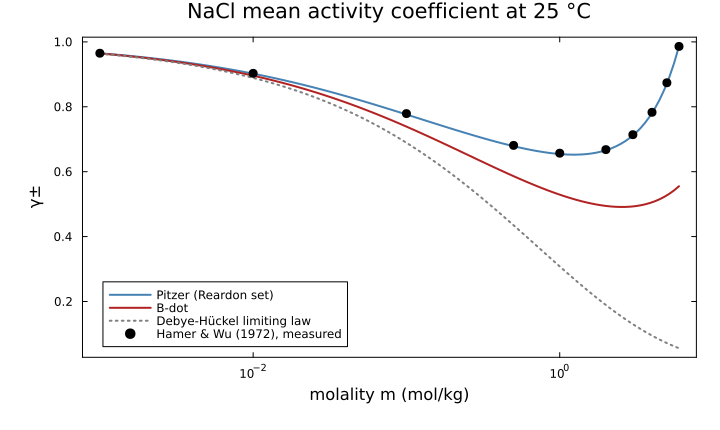
Read on a logarithmic axis, the three models are one curve below a millimolal — they must be, the limiting law is exact there — and separate irreversibly above a hundredth molal. The measured points sit on the Pitzer curve throughout.
p2 = plot(ms, [100 * (γ_of(lna_pz, m) - 1) * 0 for m in ms];
    label = "", color = :black, linewidth = 1, linestyle = :dash,
    xscale = :log10, xlabel = "molality m (mol/kg)",
    ylabel = "deviation from measurement (%)",
    title = "Where each model leaves the data", legend = :bottomleft)
scatter!(p2, [h[1] for h in HW], [100 * (γ_of(lna_pz, h[1]) - h[3]) / h[3] for h in HW];
    label = "Pitzer", color = :steelblue, markersize = 5)
scatter!(p2, [h[1] for h in HW], [100 * (γ_of(lna_bd, h[1]) - h[3]) / h[3] for h in HW];
    label = "B-dot", color = :firebrick, markersize = 5, markershape = :diamond)
hline!(p2, [-1, 1]; label = "± 1 %", color = :seagreen, linestyle = :dot)
plot(p2; size = (720, 430), left_margin = 10Plots.mm, bottom_margin = 8Plots.mm)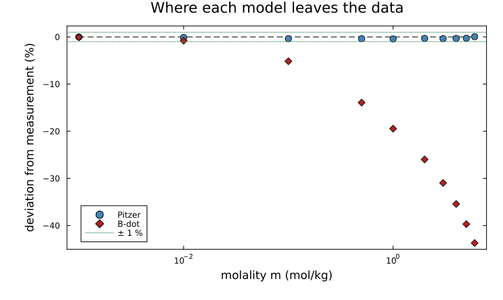
This is also, incidentally, a check on the transcription of the parameter file: the Na/Cl coefficients were read off a scanned table, and nothing mistyped reproduces a measured curve over four decades.
3. The dilute limit, exactly
A model that expands around ideality has no freedom as the solution empties: log₁₀ γ± → −A|z₊z₋|√I, and this is the check a mistyped coefficient cannot survive either.
println("       m        ln γ± (Pitzer)    limiting law     ratio")
for m in (1.0e-6, 1.0e-5, 1.0e-4, 1.0e-3)
    out = lna_pz([n_w, m, m], prm(3))
    lnγ = ((out[2] - log(m)) + (out[3] - log(m))) / 2
    law = -A25 * sqrt(m) * log(10)
    @printf("  %8.1e    %14.6f  %14.6f  %8.4f\n", m, lnγ, law, lnγ / law)
end
m ln γ± (Pitzer) limiting law ratio
1.0e-06 -0.001176 -0.001177 0.9987
1.0e-05 -0.003707 -0.003724 0.9957
1.0e-04 -0.011614 -0.011775 0.9864
1.0e-03 -0.035665 -0.037236 0.95784. Gibbs-Duhem, exactly
The reason to prefer this model.
μ_pz = build_potentials(nacl, model)
μ_bd = build_potentials(nacl, HKFActivityModel())

function gd(mu, m, dn)
    n0 = [n_w, m, m]
    dμ = ForwardDiff.jacobian(nn -> mu(nn, prm(3)), n0) * dn
    return abs(sum(n0 .* dμ)) / max(norm(n0 .* abs.(dμ)), 1.0)
end

println("                          Pitzer        B-dot")
for (name, dn) in ("dissolution  " => [0.0, 1.0, 1.0],
                   "ion exchange " => [0.0, 1.0, -1.0],
                   "water removal" => [-1.0, 0.0, 0.0])
    for m in (0.1, 1.0, 3.0)
        @printf("  %s m = %4.1f   %10.3e   %10.3e\n",
                name, m, gd(μ_pz, m, dn), gd(μ_bd, m, dn))
    end
end
Pitzer B-dot
dissolution m = 0.1 9.890e-17 6.916e-06
dissolution m = 1.0 0.000e+00 6.661e-05
dissolution m = 3.0 0.000e+00 1.081e-04
ion exchange m = 0.1 0.000e+00 8.933e-04
ion exchange m = 1.0 0.000e+00 4.275e-03
ion exchange m = 3.0 0.000e+00 6.954e-03
water removal m = 0.1 4.337e-19 2.682e-08
water removal m = 1.0 1.388e-17 2.550e-06
water removal m = 3.0 2.776e-17 1.492e-05Zero, at machine precision, in every direction and at every molality — against a B-dot residual that grows with concentration. No fit was involved in either column; the difference is structural.
5. What the set refuses, and why that is correct
A Pitzer model cannot fall back on ideal behavior for one pair, so completeness is checked when the model meets a species list, and the error names what is missing:
with_br = ChemicalSystem(
    [dict[s] for s in split("H2O@ Na+ Cl- Br-")], ["H2O@", "Na+", "Cl-", "Br-"]
)
try
    activity_model(with_br, model)
catch err
    println(first(split(err.msg, ". ")), ".")
end
PitzerActivityModel: the parameter set has no beta0 for 1 cation-anion pair(s) this system contains: Na+/Br-.The same mechanism refuses something more important. A Pitzer set assumes the speciation it was fitted with, and Reardon's is fully dissociated: the association of Ca with SO₄, of Na with OH, is inside the
cem = build_species(datapath("cemdata18-thermofun.json"); verbose = false)
pairs_present = [
    symbol(s) for s in cem
        if symbol(s) in ("Ca(SO4)@", "CaOH+", "Na(SO4)-", "K(SO4)-", "NaOH@", "KOH@",
                         "Na(CO3)-", "MgSO4@", "HSiO3-", "SiO2@")
]
println("ion pairs and silica species CEMDATA18 carries: ", join(pairs_present, ", "))
┌───────────────────────────────────────────────────┐
│ Loading database: data/cemdata18-thermofun.json │
└───────────────────────────────────────────────────┘
┌────────────────────┐
│ Building species │
└────────────────────┘
Progress: 44%|██████████████████████████████████████████████████████████████████████▋ | ETA: 0:00:00[K
Progress: 84%|███████████████████████████████████████████████████████████████████████████████████████████████████████████████████████████████████████▋ | ETA: 0:00:00[K
Progress: 99%|████████████████████████████████████████████████████████████████████████████████████████████████████████████████████████████████████████████████████████████████▎| ETA: 0:00:00[K
Progress: 100%|█████████████████████████████████████████████████████████████████████████████████████████████████████████████████████████████████████████████████████████████████| Time: 0:00:00[K
ion pairs and silica species CEMDATA18 carries: SiO2@, Na(CO3)-, MgSO4@, Na(SO4)-, CaOH+, KOH@, NaOH@, Ca(SO4)@, HSiO3-, K(SO4)-So the shipped set is not a drop-in for a CEMDATA18 cement calculation, and the refusal above is the right outcome rather than a shortcoming of the implementation: a dissociated parameterization combined with an associated speciation is not a defensible calculation in any code. Using this model on a cement pore solution means building the species list the set describes — the free ions and the solids — or obtaining a parameter set fitted for the speciation at hand.
6. Where it does apply
A dissociated alkali-hydroxide-sulfate solution of the kind a cement pore solution approximates, at an ionic strength where the B-dot model is already out of its range:
pore = ChemicalSystem(
    [dict[s] for s in split("H2O@ Na+ K+ Ca+2 OH- SO4-2")],
    ["H2O@", "Na+", "K+", "Ca+2", "OH-", "SO4-2"],
)
lna_pz = activity_model(pore, PitzerActivityModel(; parameters = pars))
lna_bd = activity_model(pore, HKFActivityModel())

# a mixture in the proportions an alkali-rich pore solution reaches
n = [n_w, 0.30, 0.15, 0.02, 0.40, 0.045]
a_pz, a_bd = lna_pz(n, prm(6)), lna_bd(n, prm(6))
names = ["H2O@", "Na+", "K+", "Ca+2", "OH-", "SO4-2"]
println("            γ (Pitzer)   γ (B-dot)    ratio")
for (i, nm) in enumerate(names)
    i == 1 && continue
    m = n[i] / (n[1] * M_w)
    g_pz, g_bd = exp(a_pz[i] - log(m)), exp(a_bd[i] - log(m))
    @printf("  %-6s  %10.4f  %10.4f  %8.3f\n", nm, g_pz, g_bd, g_pz / g_bd)
end
@printf("\n  a_w:    %10.5f  %10.5f\n", exp(a_pz[1]), exp(a_bd[1]))
γ (Pitzer) γ (B-dot) ratio
Na+ 0.6711 0.5797 1.158
K+ 0.6990 0.5997 1.166
Ca+2 0.0750 0.1342 0.559
OH- 0.6587 0.5484 1.201
SO4-2 0.1395 0.1454 0.959
a_w: 0.98549 0.98632The two models disagree by tens of percent on the ions, and the disagreement is not a refinement: at this ionic strength the B-dot term is doing work it was never fitted for, while the Pitzer set was fitted over exactly this range. Which is right is a question for measurement, not for a docstring — but only one of the two is thermodynamically consistent with its own water activity, and §3 says which.
Where to go next
The derivation is in Activity models, and the API entries are PitzerParameters, build_pitzer_parameters and pitzer_origin. The next group of applications moves to surfaces, beginning with Adsorption on a single site family.