
Two families of sites, and a metal between them
Before this page
The canonical benchmark of surface complexation is hydrous ferric oxide, and the reason it is canonical is a single modeling idea: a real oxide does not offer one kind of site but two, and they differ in the two ways that matter most.
Dzombak & Morel's ferrihydrite (Dzombak and Morel, 1990) has
strong sites, 0.005 mol per mole of iron, and
weak sites, 0.2 mol per mole of iron — forty times more of them —
which share their acid-base constants exactly, and differ by nearly three orders of magnitude in how tightly they bind a metal. Neither number alone does anything interesting. Together they produce the shape every sorption experiment shows: at low loading a few strong sites take almost all the metal; once they saturate the weak ones take over, and the curve bends.
This page builds that model, sorbs zinc onto it, and compares the result with PHREEQC computing the same thing from its own database.
What this is not, yet
This runs without an electric double layer, -no_edl on both sides. The published Dzombak & Morel calibration assumes a diffuse layer, so these constants are being used outside the model they were fitted in. That is legitimate as a cross-code check — the two codes are doing the same thing — and it is not a reproduction of the published titration. The layer is switched on at the end of this page, which is that reproduction; it is kept apart because comparing two codes on one model and comparing a model with and without its double layer are two different questions.
The two families
Both hang from one support, and each carries its own pseudo-element, its own budget and its own mixing.
using ChemistryLab, DynamicQuantities, SciMLBase

const RT = R_GAS * 298.15
g0(v) = SymbolicFunc(v * u"J/mol")
mRT(logK) = -RT * log(10.0^logK)

# PHREEQC's own constants for this model.
logK_prot, logK_depr = 7.29, -8.93
logK_Zn_strong, logK_Zn_weak = 0.99, -1.99

# The aqueous species come from a database the package ships, not from numbers
# typed here — see [Where the numbers come from](@ref sec-manual-numbers).
db = Dict(symbol(s) => s for s in
          build_species(datapath("slop98-inorganic-thermofun.json"); verbose = false))
h2o, hp, oh = db["H2O@"], db["H+"], db["OH-"]
zn, na, cl = db["Zn+2"], db["Na+"], db["Cl-"]
G(s) = ustrip(us"J/mol", s[:ΔₐG⁰](T = 298.15u"K", P = 1.0e5u"Pa"; unit = true))

# Only the SURFACE species are built here, and only because no database carries
# them: their standard energies are constructed to *be* the log K above. The
# zinc complexes carry the aqueous zinc's own energy, because
# XsOH + Zn²⁺ = XsOZn⁺ + H⁺ puts it in the balance.
sf(sym, g) = (s = Species(sym; aggregate_state = AS_SURFACE, class = SC_SURFCOMPLEX);
              s[:ΔₐG⁰] = g0(g); s)

s_free, s_prot = sf("XsOH", 0.0), sf("XsOH2+", mRT(logK_prot))
s_depr, s_zn   = sf("XsO-", mRT(logK_depr)), sf("XsOZn+", mRT(logK_Zn_strong) + G(zn))
w_free, w_prot = sf("XwOH", 0.0), sf("XwOH2+", mRT(logK_prot))
w_depr, w_zn   = sf("XwO-", mRT(logK_depr)), sf("XwOZn+", mRT(logK_Zn_weak) + G(zn))

n_Fe = 1.0e-3
N_strong, N_weak, Zn_total = 0.005n_Fe, 0.2n_Fe, 1.0e-5

support = SurfaceSupport("hydrous ferric oxide", nothing, FixedSurfaceArea(53.4))
fam_s = SiteFamily("Hfo_s", s_free, [s_prot, s_depr, s_zn];
                   capacity = TotalSiteAmount(N_strong * u"mol"), support)
fam_w = SiteFamily("Hfo_w", w_free, [w_prot, w_depr, w_zn];
                   capacity = TotalSiteAmount(N_weak * u"mol"), support)
(fam_s, fam_w)
(SiteFamily("Hfo_s", :Xs, 4 members, TotalSiteAmount on hydrous ferric oxide), SiteFamily("Hfo_w", :Xw, 4 members, TotalSiteAmount on hydrous ferric oxide))The two differ in their symbol, their budget and their zinc affinity. They differ in nothing else — the protonation and deprotonation constants are the same object twice.
The system
species = [h2o, hp, oh, zn, na, cl,
           s_free, s_prot, s_depr, s_zn, w_free, w_prot, w_depr, w_zn]
cs = ChemicalSystem(species, [h2o, hp, zn, na, cl, s_free, w_free];
                    site_families = [fam_s, fam_w])
cs.site_groups           # two groups, free site first in each
2-element Vector{Vector{Int64}}:
[7, 8, 9, 10]
[11, 12, 13, 14]Each family gets its own conservation row, and each is closed on its own members. Two families on one support share the mineral, not the budget.
i = Dict(symbol(sp) => k for (k, sp) in enumerate(cs.species))
n0 = Any[fill(1.0e-14u"mol", length(cs.species))...]
n0[i["H2O@"]] = ustrip(us"mol", 1.0u"kg" / h2o[:M]) * u"mol"   # one kilogram
n0[i["Na+"]] = 0.01u"mol"; n0[i["Cl-"]] = 0.01u"mol"
n0[i["Zn+2"]] = Zn_total * u"mol"
n0[i["XsOH"]] = N_strong * u"mol"; n0[i["XwOH"]] = N_weak * u"mol"
state = ChemicalState(cs, n0)

des = DualEquilibriumSolver(cs, DaviesActivityModel())
b = Float64.(cs.SM.A) * Float64[ustrip(us"mol", x) for x in state.n]

function at(pH)
    eq = SciMLBase.solve(des, state; b = b, constraint = FixedpH(pH))
    n = Float64[ustrip(us"mol", x) for x in eq.n]
    return (strong = n[i["XsOZn+"]] / Zn_total,
            weak   = n[i["XwOZn+"]] / Zn_total,
            free   = n[i["Zn+2"]] / Zn_total)
end
at(7.0)
(strong = 0.47711494160716533, weak = 0.42728919892106076, free = 0.09559586148024775)At pH 7, nine tenths of the zinc is on the surface — and half of it sits on sites that are forty times scarcer. That is what a thousandfold affinity buys.
The edge
[(pH, round.(values(at(pH)); digits = 4)) for pH in 5.0:1.0:8.0]4-element Vector{Tuple{Float64, Tuple{Float64, Float64, Float64}}}:
(5.0, (0.0157, 0.0007, 0.9836))
(6.0, (0.3319, 0.0413, 0.6268))
(7.0, (0.4771, 0.4273, 0.0956))
(8.0, (0.4809, 0.514, 0.0051))Read the three columns across the rows. The strong sites fill first and stop: they run out. The weak sites keep going, and by pH 8 they carry most of the load simply because there are more of them.
using Plots

# PHREEQC's answer, from test/surface_complexation.jl
PHREEQC_PH     = [4.0, 5.0, 6.0, 7.0, 8.0, 9.0]
PHREEQC_SORBED = [0.00017033047684235052, 0.016218434554914892, 0.37188533609051405, 0.9028626468821174, 0.9939171294298249, 0.991222704808546]

pHs = range(4, 9; length = 60)
d = [at(pH) for pH in pHs]
p = plot(; xlabel = "pH", ylabel = "fraction of the zinc",
         title = "Zinc on hydrous ferric oxide, no double layer",
         legend = :left, ylims = (-0.02, 1.02))
plot!(p, pHs, [x.strong for x in d]; label = "on strong sites", color = :firebrick, lw = 2)
plot!(p, pHs, [x.weak for x in d];   label = "on weak sites",   color = :seagreen,  lw = 2)
plot!(p, pHs, [x.free for x in d];   label = "in solution",     color = :steelblue, lw = 2)
scatter!(p, PHREEQC_PH, PHREEQC_SORBED; label = "PHREEQC, total sorbed",
         color = :black, markersize = 5, markerstrokewidth = 0)
plot!(p, pHs, [x.strong + x.weak for x in d]; label = "total sorbed",
      color = :black, linestyle = :dash, lw = 2)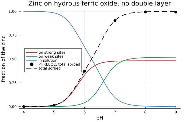
The strong-site curve is the one to watch. It rises first and steeply — a thousandfold affinity wins the early competition outright, scarcity notwithstanding — and then stops flat at 0.48. Nothing about the chemistry changed there: it ran out of sites. There are 5 µmol of strong sites for 10 µmol of zinc, so they cannot hold more than half of it however favorable the reaction, and the plateau sits just under that ceiling because protons occupy the rest.
Everything above that plateau is the weak sites, which take over precisely because the strong ones are full. A single-site model produces neither the early steepness nor the ceiling — it would give one sigmoid, and the experiment does not.
Against PHREEQC, and what the difference is
The black points are PHREEQC running the same model from its own database. They sit on the dashed curve, and the worst departure across the edge is 0.94 %.
That is a hundred times worse than the protolysis comparison, which agrees to 1.7 × 10⁻⁸, and the reason is instructive: the difference is not in the surface model.
Zinc carries two charges, so its activity coefficient leaves 1 quickly — about 0.72 at an ionic strength of 0.01 by the Davies equation. A model that puts it at 1 says the metal is more available than it is, and drives more sorption. Running the identical system under both aqueous models turns that explanation into a measurement:
| aqueous model | worst departure from PHREEQC |
|---|---|
| ideal (dilute) | 49 % |
| Davies | 0.94 % |
A factor of fifty, from changing nothing but what the aqueous phase does. The 0.94 % that remains is the distance between Davies and PHREEQC's own extended Debye-Hückel — two aqueous models, neither of them this package's surface model.
That is also why the protolysis comparison was built without a metal: with only protons involved, and the proton activity prescribed on both sides, no aqueous activity coefficient enters at all, and the surface chemistry is compared alone. test/surface_complexation.jl keeps both comparisons for that reason.
The same edge, with the double layer
Everything above ran -no_edl. Dzombak & Morel's constants were fitted with a diffuse layer, so this is the comparison that is actually a reproduction of the published model rather than a cross-code check on a truncated one.
Two families sit on one oxide here, and that matters as soon as there is a potential: a proton bound to a weak site charges the same surface a proton bound to a strong site does, so both feel one Ψ. The potential belongs to the support, not to the family.
using JSON
DDL = JSON.parsefile(joinpath(pkgdir(ChemistryLab), "test", "reference",
                              "phreeqc_hfo_zn_ddl.json"))
layered = SiteFamily[]   # the same two families, with the layer on
for (name, free, others, N) in (
        ("Hfo_s", s_free, [s_prot, s_depr, s_zn], N_strong),
        ("Hfo_w", w_free, [w_prot, w_depr, w_zn], N_weak),
    )
    push!(layered, SiteFamily(name, free, others; capacity = TotalSiteAmount(N),
                              support, model = DiffuseLayer(; area = 53.4)))
end
cs_dl = ChemicalSystem(species, [h2o, hp, zn, na, cl, s_free, w_free];
                       site_families = layered)
j = Dict(symbol(sp) => k for (k, sp) in enumerate(cs_dl.species))
des_dl = DualEquilibriumSolver(cs_dl, DaviesActivityModel())

function sorbed_with_layer(pt)
    n0 = Any[fill(1.0e-14u"mol", length(cs_dl.species))...]
    n0[j["H2O@"]] = ustrip(us"mol", 1.0u"kg" / h2o[:M]) * u"mol"
    n0[j["Na+"]] = 0.01u"mol"
    # the chloride carries PHREEQC's own titrant, so the ionic strengths match
    n0[j["Cl-"]] = (2 * pt["I"] - 0.01 - 10.0^(-pt["pH"]) - 10.0^(pt["pH"] - 14))u"mol"
    n0[j["Zn+2"]] = Zn_total * u"mol"
    n0[j["XsOH"]] = N_strong * u"mol"; n0[j["XwOH"]] = N_weak * u"mol"
    st = ChemicalState(cs_dl, n0)
    bb = Float64.(cs_dl.SM.A) * Float64[ustrip(us"mol", x) for x in st.n]
    eq = SciMLBase.solve(des_dl, st; b = bb, constraint = FixedpH(pt["pH"]))
    n = Float64[ustrip(us"mol", x) for x in eq.n]
    return (n[j["XsOZn+"]] + n[j["XwOZn+"]]) / Zn_total
end

using Printf
println("  pH   no layer   with layer   PHREEQC (layer)")
for pt in DDL["points"]
    a = at(pt["pH"])
    @printf("%5.1f %10.4f %12.4f %16.4f\n",
            pt["pH"], a.strong + a.weak, sorbed_with_layer(pt),
            pt["zn_sorbed_fraction"])
end
pH no layer with layer PHREEQC (layer)
4.0 0.0002 0.0001 0.0001
5.0 0.0164 0.0057 0.0056
6.0 0.3732 0.1825 0.1816
7.0 0.9044 0.7094 0.7069
8.0 0.9949 0.9921 0.9907
9.0 0.9991 0.9999 0.9990The layer moves the edge by about half a pH unit — at pH 6 the sorbed fraction falls from 0.37 to 0.18 — which is why a calibration made with it cannot be used without it. The middle column follows the right-hand one to 0.5 %, slightly better than the 0.94 % of the comparison without the layer.
See also
A charged surface, screened — the same layer on the acid-base half, across three ionic strengths, and why the potential is carried as an unknown.
Adsorption on a single site family — the same machinery on one family, against a closed form.
Chemistry that happens on a surface — where the electrostatic models are derived and what each costs the certificate.