Adsorption on a single site family

Before this page

Chemistry that happens on a surface §1 to §4, and Surface areas for the syntax.

The smallest complete surface calculation: one family of sites on an oxide, titrated by pH. It is small enough to check by hand, and it exercises everything the surface model does — a site budget, a conservation row, ideal mixing on that budget, and competition between two occupied states for one finite capacity.

The physics is the acid-base behavior of an oxide surface. A hydroxyl group exposed on the grain takes a proton in acid and gives one up in base:

so the surface is positive in acid, negative in base, and neutral in between. The constants below are Dzombak & Morel's for the weak sites of hydrous ferric oxide (Dzombak and Morel, 1990), log K = 7.29 and log K = −8.93, the values PHREEQC ships.

The species

A surface species is an ordinary species. What marks it is its aggregate state, and the site symbol in its formula — Xs here — which is what turns the site balance into a row of the conservation matrix.

using ChemistryLab, DynamicQuantities, SciMLBase

const RT = R_GAS * 298.15
g0(v) = SymbolicFunc(v * u"J/mol")          # a constant standard energy

logK₁, logK₂ = 7.29, -8.93                  # protonation, deprotonation

free = Species("XsOH"; aggregate_state = AS_SURFACE, class = SC_SURFCOMPLEX)
free[:ΔₐG⁰] = g0(0.0)                       # the reference state of the family

prot = Species("XsOH2+"; aggregate_state = AS_SURFACE, class = SC_SURFCOMPLEX)
prot[:ΔₐG⁰] = g0(-RT * log(10.0^logK₁))     # ΔrG° = −RT ln K

depr = Species("XsO-"; aggregate_state = AS_SURFACE, class = SC_SURFCOMPLEX)
depr[:ΔₐG⁰] = g0(-RT * log(10.0^logK₂))

atoms(free)

OrderedCollections.OrderedDict{Symbol, Int64} with 3 entries:
  :Xs => 1
  :O  => 1
  :H  => 1

Xs is the family; O and H are real atoms, and they are the only ones that weigh anything — the support is weighed once, by its own mineral species.

free[:M]        # an oxygen and a hydrogen: the adsorbed part alone

0.017006999994122744 kg mol⁻¹

The surface, and its budget of sites

# The aqueous species come from a database the package ships, not from numbers
# typed here — see [Where the numbers come from](@ref sec-manual-numbers).
db = Dict(symbol(s) => s for s in
          build_species(datapath("slop98-inorganic-thermofun.json"); verbose = false))
h2o, hp, oh = db["H2O@"], db["H+"], db["OH-"]

N_sites = 2.0e-4                               # mol of sites
support = SurfaceSupport("hydrous ferric oxide", nothing, FixedSurfaceArea(600.0))
family  = SiteFamily("Hfo_w", free, [prot, depr];
                     capacity = TotalSiteAmount(N_sites * u"mol"), support)

SiteFamily("Hfo_w", :Xs, 3 members, TotalSiteAmount on hydrous ferric oxide)

TotalSiteAmount is the honest description of a batch experiment: a weighed sorbent, a known number of sites. The two other forms — a density per square meter, a capacity per kilogram — exist because published data comes in both, and converting between them would need an area nobody measured.

The system, and the row that makes it a surface

The free site is the primary. That is not a matter of taste: a bare site species in its place is inconsistent in charge with a neutral free site, which silently adds a spurious charge component to the matrix.

species = [h2o, hp, oh, free, prot, depr]
cs = ChemicalSystem(species, [h2o, hp, free]; site_families = [family])
row = cs.SM.A[findfirst(p -> symbol(p) == "XsOH", cs.SM.primaries), :]
Int.(row)

6-element Vector{Int64}:
 0
 0
 0
 1
 1
 1

One per surface species, zero on every aqueous one. That row is

and it was produced by the same matrix assembly that writes every other conservation law. Nothing was special-cased for it.

One point

Start with every site free, and hold the pH at 6.

n0 = Any[fill(1.0e-12u"mol", length(cs.species))...]
n0[1] = ustrip(us"mol", 1.0u"kg" / h2o[:M]) * u"mol"   # exactly one kilogram
n0[4] = N_sites * u"mol"
state = ChemicalState(cs, n0)

des = DualEquilibriumSolver(cs, DiluteSolutionModel())
b   = Float64.(cs.SM.A) * Float64[ustrip(us"mol", x) for x in state.n]

eq = SciMLBase.solve(des, state; b = b, constraint = FixedpH(6.0))
n  = Float64[ustrip(us"mol", x) for x in eq.n]
N  = n[4] + n[5] + n[6]
(free = n[4] / N, protonated = n[5] / N, deprotonated = n[6] / N)

(free = 0.04878138991523251, protonated = 0.9511612969490296, deprotonated = 5.731313573786146e-5)

At pH 6 the surface is mostly protonated, and almost none of it is deprotonated — the second reaction's constant is nearly three orders of magnitude below the proton activity that would drive it.

Against the closed form

The point of the exercise. Eliminating the free site from the two mass-action laws and the site balance gives the competitive Langmuir form, derived in the theory page:

Both drives come from the same proton activity, which is why one constraint is enough to test competition.

function solved(pH)
    eq = SciMLBase.solve(des, state; b = b, constraint = FixedpH(pH))
    n = Float64[ustrip(us"mol", x) for x in eq.n]
    N = n[4] + n[5] + n[6]
    return (n[4] / N, n[5] / N, n[6] / N)
end

function closed_form(pH)
    a_H = 10.0^(-pH)
    β = (10.0^logK₁ * a_H, 10.0^logK₂ / a_H)
    d = 1 + sum(β)
    return (1 / d, β[1] / d, β[2] / d)
end

worst = 0.0
for pH in 4.0:1.0:9.0
    s, c = solved(pH), closed_form(pH)
    global worst = max(worst, maximum(abs.(s ./ c .- 1)))
end
worst      # worst relative departure from the closed form, over six pH values

1.6604378094697836e-8

That is the solver and the algebra agreeing to the last digits either can claim. No isotherm was written: Langmuir is what a conservation law and a mass-action law produce together.

Conservation, checked on its own scale

A residual is only meaningful against something. Water, a trace species and a site budget differ by ten orders of magnitude, so each conserved quantity is scaled by how much matter its own row moves.

A = Float64.(cs.SM.A)
eq_closed = SciMLBase.solve(des, state; b = b)          # no constraint: closed
nc = Float64[ustrip(us"mol", x) for x in eq_closed.n]
r  = A * nc .- b
turnover(c) = sum(abs(A[c, i]) * nc[i] for i in eachindex(nc))
[(symbol(p), abs(r[c]) / max(abs(b[c]), turnover(c))) for (c, p) in enumerate(cs.SM.primaries)]

3-element Vector{Tuple{String, Float64}}:
 ("H2O@", 1.536051285635328e-15)
 ("H+", 7.036474912913334e-12)
 ("XsOH", 3.9952714129695915e-11)

The site row is conserved to the same precision as the water it sits in.

The titration curve

using Plots

pHs = range(3, 11; length = 200)
curves = [solved(pH) for pH in pHs]
exact  = [closed_form(pH) for pH in pHs]

p = plot(;
    xlabel = "pH", ylabel = "fraction of sites",
    title  = "An amphoteric surface, one family of sites",
    legend = :right, ylims = (-0.02, 1.02),
)
for (k, (lab, col)) in enumerate((
        ("≡XOH  (free)", :steelblue),
        ("≡XOH₂⁺ (protonated)", :firebrick),
        ("≡XO⁻  (deprotonated)", :seagreen),
    ))
    plot!(p, pHs, [c[k] for c in exact];
          label = "$lab — closed form", color = col, linewidth = 2)
    scatter!(p, pHs[1:12:end], [c[k] for c in curves[1:12:end]];
             label = "$lab — solved", color = col, markersize = 4, markerstrokewidth = 0)
end
p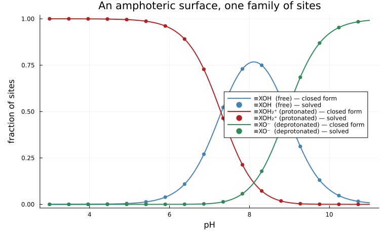

The two curves of each color are one curve.

Three features are worth reading off it, because each is the closed form made visible:

• the protonated fraction falls through one half near pH = log K₁ = 7.29, and the deprotonated one rises through one half near pH = −log K₂ = 8.93. Near, not at: with three states sharing one budget the half-point is pulled slightly by the third, to 0.494 rather than 0.500. A two-state model would put them exactly at the pK, and that small difference is the shared denominator doing its work;

• the free fraction peaks at pH = (log K₁ − log K₂)/2 = 8.11, where the two drives are equal. Its height, 1/(1 + 2\sqrt{K_1 K_2}) = 0.768, is not one: even at its most neutral the surface is a quarter occupied, because both reactions still run;

• that same pH, where the positive and negative states are equally populated, is the point of zero charge.

And against another code

The same calculation is checked against PHREEQC, running Dzombak & Morel's model from its own database, in test/surface_complexation.jl. The comparison is made at matched proton activity — which both codes prescribe exactly — so the aqueous activity models, which differ, do not enter. With no metal in the system there is nothing else they could enter through.

The worst relative departure over the six pH values is 1.7 × 10⁻⁸.

See also

• Chemistry that happens on a surface — where the closed form above comes from, and what the model does not cover.

• Surface areas — the syntax in full, including the three ways a site budget can be specified.