
Getting started
This page takes a first calculation from installation to a solved equilibrium in three steps: the thermodynamic data of a few species are read from a database distributed with the package, the reaction between them is written and its equilibrium constant evaluated, and the equilibrium of calcite with water is finally computed. No knowledge of chemical thermodynamics is assumed. Each quantity is defined in the chapter Theory, to which the text refers at the point where the quantity is first needed.
Installation
ChemistryLab.jl is registered in the General registry and is installed with the Julia package manager, either from the Pkg mode of the REPL (entered by typing ])
pkg> add ChemistryLabor, equivalently, through the Pkg API:
julia> import Pkg; Pkg.add("ChemistryLab")A first reaction: calcite in water
The dissolution of calcite is written
and its equilibrium constant
where
The species are read from CEMDATA18 (Lothenbach et al., 2019), a database for cement systems whose file is distributed with the package as a copy of the one maintained on ThermoHub. build_species reads the file and returns a vector of species whose thermodynamic functions are already compiled; speciation then keeps the species whose elements are all found among those of a few seed species, here calcium, carbon, hydrogen and oxygen from Cal, H2O@ and CO2. The three aqueous gases listed in exclude_species are left out because their presence would open a redox equilibrium that this example does not need.
using ChemistryLab
using DynamicQuantities # for unit management

all_species = build_species(datapath("cemdata18-thermofun.json"); verbose = false)
species_calcite = speciation(all_species, split("Cal H2O@ CO2");
                             aggregate_state=[AS_AQUEOUS],
                             exclude_species=split("H2@ O2@ CH4@"))
dict_species_calcite = Dict(symbol(s) => s for s in species_calcite)
Dict{String, Species{Int64}} with 12 entries:
"Ca(HCO3)+" => Ca(HCO3)+ {CaHCO3+} [Ca(HCO3)+ ◆ Ca(HCO₃)⁺]
"CaOH+" => CaOH+ {CaOH+} [Ca(OH)+ ◆ Ca(OH)⁺]
"HCO3-" => HCO3- {HCO3-} [HCO3- ◆ HCO₃⁻]
"H+" => H+ {H+} [H+ ◆ H⁺]
"CO2@" => CO2@ {CO2 aq} [CO2@ ◆ CO₂@]
"Ca(CO3)@" => Ca(CO3)@ {CaCO3 aq} [CaCO3@ ◆ CaCO₃@]
"CO3-2" => CO3-2 {CO3-2} [CO3-2 ◆ CO₃²⁻]
"CO2" => CO2 {CO2 g} [CO2 ◆ CO₂]
"Cal" => Cal {Calcite} [CaCO3 ◆ CaCO₃]
"Ca+2" => Ca+2 {Ca+2} [Ca+2 ◆ Ca²⁺]
"OH-" => OH- {OH-} [OH- ◆ OH⁻]
"H2O@" => H2O@ {H2O l} [H2O@ ◆ H₂O@]Each species carries its molar mass and its standard thermodynamic functions of temperature: heat capacity, entropy, enthalpy and Gibbs energy. They can be inspected and plotted directly.
dict_species_calcite["Cal"]Species{Int64}
name: Calcite
symbol: Cal
formula: CaCO3 ◆ CaCO₃
atoms: Ca => 1, C => 1, O => 3
charge: 0
aggregate_state: AS_CRYSTAL
class: SC_COMPONENT
properties: M = 0.10008599996541243 kg mol⁻¹
Tref = 298.15 K
Pref = 100000.0 m⁻¹ kg s⁻²
Cp⁰ = 104.5163192749 + 0.02192415855825T + -2.59408e6 / (T^2) [m² kg s⁻² K⁻¹ mol⁻¹] ◆ vars=(T) ◆ T=298.15 K
ΔₐH⁰ = -1.2482415842895252e6 + 104.5163192749T + 2.59408e6 / T + 0.010962079279125(T^2) [m² kg s⁻² mol⁻¹] ◆ vars=(T) ◆ T=298.15 K
S⁰ = -523.9438829693111 + 0.02192415855825T + 104.5163192749log(T) + 1.29704e6 / (T^2) [m² kg s⁻² K⁻¹ mol⁻¹] ◆ vars=(T) ◆ T=298.15 K
ΔₐG⁰ = -1.1423813547027335e6 + 628.460202244211T + 1.29704e6 / T - 0.010962079279125(T^2) - 104.5163192749T*log(T) [m² kg s⁻² mol⁻¹] ◆ vars=(T) ◆ T=298.15 K
V⁰ = 3.6933999061584004e-5 [m³ mol⁻¹]
Cp⁰_Tref = 81.87109375 m² kg s⁻² K⁻¹ mol⁻¹
ΔₐH⁰_Tref = -1.207405e6 m² kg s⁻² mol⁻¹
S⁰_Tref = 92.675598144531 m² kg s⁻² K⁻¹ mol⁻¹
ΔₐG⁰_Tref = -1.129176e6 m² kg s⁻² mol⁻¹
V⁰_Tref = 3.6933999061584004e-5 m³ mol⁻¹using Plots
p1 = plot(xlabel="Temperature [°C]", ylabel="Cp⁰ [J/mol/K]", title="Heat capacity of calcite \nas a function of temperature")
plot!(p1, θ -> dict_species_calcite["Cal"].Cp⁰(T = θ*ua"degC"), 0:0.1:100, label="Cp⁰")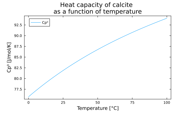
Writing the reactions requires a choice of independent species, the primaries, in terms of which every other species is expressed. The stoichiometric matrix collects those decompositions, one column per species and one row per primary; its construction is detailed in Stoichiometric matrices.
primaries = [dict_species_calcite[s] for s in split("H2O@ H+ CO3-2 Ca+2")]
SM = StoichMatrix(collect(values(dict_species_calcite)), primaries)
pprint(SM)
┌───────┬───────────┬───────┬───────┬────┬──────┬──────────┬───────┬─────┬─────┬──────┬─────┬──────┐
│ │ Ca(HCO3)+ │ CaOH+ │ HCO3- │ H+ │ CO2@ │ Ca(CO3)@ │ CO3-2 │ CO2 │ Cal │ Ca+2 │ OH- │ H2O@ │
├───────┼───────────┼───────┼───────┼────┼──────┼──────────┼───────┼─────┼─────┼──────┼─────┼──────┤
│ H2O@ │ │ 1 │ │ │ -1 │ │ │ -1 │ │ │ 1 │ 1 │
│ H+ │ 1 │ -1 │ 1 │ 1 │ 2 │ │ │ 2 │ │ │ -1 │ │
│ CO3-2 │ 1 │ │ 1 │ │ 1 │ 1 │ 1 │ 1 │ 1 │ │ │ │
│ Ca+2 │ 1 │ 1 │ │ │ │ 1 │ │ │ 1 │ 1 │ │ │
└───────┴───────────┴───────┴───────┴────┴──────┴──────────┴───────┴─────┴─────┴──────┴─────┴──────┘The reactions follow from the matrix, each carrying its own thermodynamic functions of temperature, among which the equilibrium constant.
list_reactions = reactions(SM)
dict_reactions_calcite = Dict(r.symbol => r for r in list_reactions)
Dict{String, Reaction{Species{Int64}, Int64, Species{Int64}, Int64, Int64}} with 8 entries:
"Ca(HCO3)+" => H⁺ + CO₃²⁻ + Ca²⁺ = Ca(HCO₃)⁺
"Cal" => CO₃²⁻ + Ca²⁺ = CaCO₃
"CO2@" => 2H⁺ + CO₃²⁻ = CO₂@ + H₂O@
"CaOH+" => H₂O@ + Ca²⁺ = Ca(OH)⁺ + H⁺
"OH-" => H₂O@ = OH⁻ + H⁺
"HCO3-" => H⁺ + CO₃²⁻ = HCO₃⁻
"Ca(CO3)@" => CO₃²⁻ + Ca²⁺ = CaCO₃@
"CO2" => 2H⁺ + CO₃²⁻ = CO₂ + H₂O@dict_reactions_calcite["Cal"].logK⁰NumericFunc:
Unit: [m² kg s⁻² mol⁻¹]
Variables: T, P
References: T=298.15 K, P=100000.0 m⁻¹ kg s⁻²p2 = plot(xlabel="Temperature [°C]", ylabel="pKs", title="Solubility product (pKs) of calcite \nas a function of temperature")
plot!(p2, θ -> dict_reactions_calcite["Cal"].logK⁰(T = θ*ua"degC"), 0:0.1:100, label="pKs")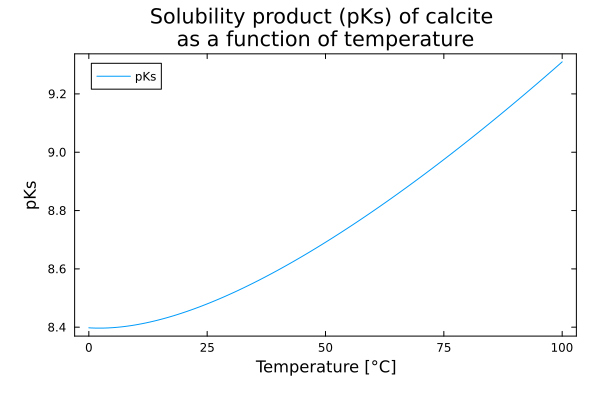
A first equilibrium
The previous section evaluated a property of one reaction. Solving the equilibrium of a system is a different question: the amounts of all species are sought that minimize the Gibbs energy of the system under the conservation of its elements. Three objects are involved.
| object | role |
|---|---|
ChemicalSystem | the immutable description of the system: species, primaries, stoichiometric matrices; built once and reused |
ChemicalState | the mutable state: amounts in mol, temperature and pressure |
equilibrate | the solver, which tries every available route and returns the state that optimality_certificate proves to be the minimum; equilibrate_certified returns the certificate as well |
using Optimization, OptimizationIpopt
using DynamicQuantities

# ChemicalSystem: declare the species and which four are the independent basis
primaries_eq = [dict_species_calcite[s] for s in split("H2O@ H+ CO3-2 Ca+2")]
cs = ChemicalSystem(collect(values(dict_species_calcite)), primaries_eq)

# ChemicalState: set the initial amounts
state = ChemicalState(cs)
set_quantity!(state, "Cal",  1e-3u"mol")   # 1 mmol of calcite
set_quantity!(state, "H2O@", 1.0u"kg")     # 1 kg of water

# Seed H⁺ and OH⁻ at pH 4 (trace amounts to help convergence)
V = volume(state)
set_quantity!(state, "H+",  1e-4u"mol/L" * V.liquid)
set_quantity!(state, "OH-", 1e-10u"mol/L" * V.liquid)

# Solve: find the Gibbs-energy minimum
state_eq = equilibrate(state)
┌ Warning: Verbosity toggle: missing_second_order_ad
│ The selected optimization algorithm requires second order derivatives, but `SecondOrder` ADtype was not provided. So a `SecondOrder` with AutoForwardDiff() for both inner and outer will be created, this can be suboptimal and not work in some cases so an explicit `SecondOrder` ADtype is recommended.
└ @ OptimizationBase ~/.julia/packages/OptimizationBase/BEgWO/src/cache.jl:116The solved state in full — every species, with its amount
state_eqChemicalState{Species{Int64}, AbstractReaction, DynamicQuantities.Quantity{Float64, DynamicQuantities.SymbolicDimensions{DynamicQuantities.FRInt32}}, Float64}
┌─────────────────────────────────────────────────────────────────────────────────────────────────────────────────────┐
│ T : 298.15 K │
│ P : 1.0 bar │
╞═════════════════════════════════════════════════════════════════════════════════════════════════════════════════════╡
│ # liquid #│ n [mol]│ m [g]│ V [cm³]│ c [mol/L]│ │
├┄┄┄┄┄┄┄┄┄┄┄┄┄┄┄┄┄┄┄┄┄┄┄┄┄┄┄┄┄┄┄┄┄┄┄┄┄┄┄┄┄┄┄┄┄┄┄┄┄┄┄┄┄┄┄┄┄┄┄┄┄┄┄┄┄┄┄┄┄┄┄┄┄┄┄┄┄┄┄┄┄┄┄┄┄┄┄┄┄┄┄┄┄┄┄┄┄┄┄┄┄┄┄┄┄┄┄┄┄┄┄┄┄┄┄┄┄┤
│ tot. liquid│ 55.5096│ 1000.02│ 1002.96│ │ │
├┄┄┄┄┄┄┄┄┄┄┄┄┄┄┄┄┄┄┄┄┄┄┄┄┄┄┄┄┄┄┄┄┄┄┄┄┄┄┄┄┄┄┄┄┄┄┄┄┄┄┄┄┄┄┄┄┄┄┄┄┄┄┄┄┄┄┄┄┄┄┄┄┄┄┄┄┄┄┄┄┄┄┄┄┄┄┄┄┄┄┄┄┄┄┄┄┄┄┄┄┄┄┄┄┄┄┄┄┄┄┄┄┄┄┄┄┄┤
│ H2O@│ 55.5093│ 999.999│ 1002.96│ 55.3453│ │
│ Ca+2│ 0.000155243│ 0.00622182│ -0.00286248│ 0.000154784│ │
│ HCO3-│ 0.000133909│ 0.00817059│ 0.00324205│ 0.000133513│ │
│ OH-│ 3.39679e-5│ 0.000577693│ -0.000159916│ 3.38676e-5│ │
│ CO3-2│ 2.13327e-5│ 0.00128013│ -0.000129227│ 2.12696e-5│ │
│ Ca(CO3)@│ 5.54915e-6│ 0.000555392│ -8.68355e-5│ 5.53275e-6│ │
│ Ca(HCO3)+│ 2.65111e-7│ 2.68011e-5│ 3.53387e-6│ 2.64327e-7│ │
│ CO2@│ 8.86588e-8│ 3.90179e-6│ 2.9086e-6│ 8.83969e-8│ │
│ CaOH+│ 8.7515e-8│ 4.99579e-6│ 5.04303e-7│ 8.72564e-8│ │
│ H+│ 2.94308e-10│ 2.96663e-10│ 0.0│ 2.93439e-10│ │
╞═════════════════════════════════════════════════════════════════════════════════════════════════════════════════════╡
│ # solid #│ n [mol]│ m [g]│ V [cm³]│ │ │
├┄┄┄┄┄┄┄┄┄┄┄┄┄┄┄┄┄┄┄┄┄┄┄┄┄┄┄┄┄┄┄┄┄┄┄┄┄┄┄┄┄┄┄┄┄┄┄┄┄┄┄┄┄┄┄┄┄┄┄┄┄┄┄┄┄┄┄┄┄┄┄┄┄┄┄┄┄┄┄┄┄┄┄┄┄┄┄┄┄┄┄┄┄┄┄┄┄┄┄┄┄┄┄┄┄┄┄┄┄┄┄┄┄┄┄┄┄┤
│ tot. solid│ 0.000838855│ 0.0839577│ 0.0309823│ │ │
├┄┄┄┄┄┄┄┄┄┄┄┄┄┄┄┄┄┄┄┄┄┄┄┄┄┄┄┄┄┄┄┄┄┄┄┄┄┄┄┄┄┄┄┄┄┄┄┄┄┄┄┄┄┄┄┄┄┄┄┄┄┄┄┄┄┄┄┄┄┄┄┄┄┄┄┄┄┄┄┄┄┄┄┄┄┄┄┄┄┄┄┄┄┄┄┄┄┄┄┄┄┄┄┄┄┄┄┄┄┄┄┄┄┄┄┄┄┤
│ Cal│ 0.000838855│ 0.0839577│ 0.0309823│ │ │
╞═════════════════════════════════════════════════════════════════════════════════════════════════════════════════════╡
│ # gas #│ n [mol]│ m [g]│ V [cm³]│ │ p [bar]│
├┄┄┄┄┄┄┄┄┄┄┄┄┄┄┄┄┄┄┄┄┄┄┄┄┄┄┄┄┄┄┄┄┄┄┄┄┄┄┄┄┄┄┄┄┄┄┄┄┄┄┄┄┄┄┄┄┄┄┄┄┄┄┄┄┄┄┄┄┄┄┄┄┄┄┄┄┄┄┄┄┄┄┄┄┄┄┄┄┄┄┄┄┄┄┄┄┄┄┄┄┄┄┄┄┄┄┄┄┄┄┄┄┄┄┄┄┄┤
│ tot. gas│ 0.0│ 0.0│ 0.0│ │ │
├┄┄┄┄┄┄┄┄┄┄┄┄┄┄┄┄┄┄┄┄┄┄┄┄┄┄┄┄┄┄┄┄┄┄┄┄┄┄┄┄┄┄┄┄┄┄┄┄┄┄┄┄┄┄┄┄┄┄┄┄┄┄┄┄┄┄┄┄┄┄┄┄┄┄┄┄┄┄┄┄┄┄┄┄┄┄┄┄┄┄┄┄┄┄┄┄┄┄┄┄┄┄┄┄┄┄┄┄┄┄┄┄┄┄┄┄┄┤
│ CO2│ 0.0│ 0.0│ 0.0│ │ N/A│
╞═════════════════════════════════════════════════════════════════════════════════════════════════════════════════════╡
│ # TOTAL #│ n [mol]│ m [g]│ V [cm³]│ │ │
├┄┄┄┄┄┄┄┄┄┄┄┄┄┄┄┄┄┄┄┄┄┄┄┄┄┄┄┄┄┄┄┄┄┄┄┄┄┄┄┄┄┄┄┄┄┄┄┄┄┄┄┄┄┄┄┄┄┄┄┄┄┄┄┄┄┄┄┄┄┄┄┄┄┄┄┄┄┄┄┄┄┄┄┄┄┄┄┄┄┄┄┄┄┄┄┄┄┄┄┄┄┄┄┄┄┄┄┄┄┄┄┄┄┄┄┄┄┤
│ │ 55.5105│ 1000.1│ 1002.99│ │ │
╞═════════════════════════════════════════════════════════════════════════════════════════════════════════════════════╡
│ pH : 9.5299 │
│ pOH : 4.4702 │
│ porosity : 0.999969 │
│ saturation : 1.0 │
└─────────────────────────────────────────────────────────────────────────────────────────────────────────────────────┘println("pH = ", round(pH(state_eq), digits = 2))pH = 9.53The returned state gives access to every derived quantity: pH, the volumes of the phases, the amount of each species. Why the minimum exists, why it is unique, and how the solver proves that the state it returns is that minimum are explained in Proving that an answer is the answer; the options of the solver are described in Chemical Equilibrium.
Where to go next
The documentation can be entered from three directions, depending on what the reader already knows.
A reader new to chemical thermodynamics is best served by the chapter Theory read in its stated order, starting from Thermochemistry, before the Manual, which describes one kind of object per page from Species onwards.
A reader who knows what is to be computed can go to the tutorial Chemical Equilibrium, then to the aqueous examples, whose answers can be checked against closed forms, starting with CO₂ dissolution and the carbonate system.
A reader holding the oxide analysis of a cement will find the route from an analysis to a chemical system in Bogue calculation, and the worked binders from A CEM I from its clinker phases onwards.
Citing ChemistryLab
When ChemistryLab is used in published work, it is to be cited as follows.
@software{chemistrylab_jl,
  author       = {Barthélémy, Jean-François and
                  Soive, Anthony},
  title        = {ChemistryLab.jl: Numerical laboratory for
                   computational chemistry},
  doi          = {10.5281/zenodo.17756074},
  url          = {https://doi.org/10.5281/zenodo.17756074},
}