
A charged surface, screened
Before this page
Two families of sites, and a metal between them, and Chemistry that happens on a surface §8 and §9.
The zinc edge ran with the electrostatics switched off, and said in a box that the published Dzombak & Morel constants were therefore being used outside the model they were fitted in. This page closes that gap for the acid-base half of the problem, and is equally explicit about the half it does not close.
An oxide surface that binds protons becomes charged, and a charged surface is surrounded by a cloud of counter-ions that screens it. How well it is screened depends on how many ions the solution has to spare — so unlike every other quantity on these pages, the answer depends on the background electrolyte, and that dependence is the whole content of the model.
The experiment
Ferrihydrite's weak sites at Dzombak & Morel's own density — 2.0 × 10⁻⁴ mol of sites on 53.4 m², which is 2.25 sites per square nanometer — titrated from pH 4 to pH 9 in sodium chloride, at three concentrations two decades apart.
A site density is not a free parameter here
A surface a thousand times more dilute carries a thousandth of the charge per unit area, raises a potential of a few millivolts, and would let a model that did nothing at all pass for one that worked. The first draft of this comparison made exactly that mistake and reported agreement.
using ChemistryLab, DynamicQuantities, SciMLBase, OptimaSolver

const RT = R_GAS * 298.15
g0(v) = SymbolicFunc(v * u"J/mol")

# The aqueous species come from a database the package ships, not from numbers
# typed here — see [Where the numbers come from](@ref sec-manual-numbers).
const DB = Dict(symbol(s) => s for s in
                build_species(datapath("slop98-inorganic-thermofun.json"); verbose = false))

const AREA    = 53.4          # m², the support that carries the sites
const N_SITES = 2.0e-4        # mol
const LOGK    = (protonation = 7.29, deprotonation = -8.93)   # PHREEQC's own
# One kilogram of water, from the solvent's own molar mass: `55.5 mol` weighs
# 0.99983 kg, and every molality below would carry that error.
const N_WATER = ustrip(us"mol", 1.0u"kg" / DB["H2O@"][:M])

function hfo(; m_na, m_cl, model)
    h2o, hp, oh, na, cl = (DB[k] for k in ("H2O@", "H+", "OH-", "Na+", "Cl-"))

    free = Species("XsOH";   aggregate_state = AS_SURFACE, class = SC_SURFCOMPLEX); free[:ΔₐG⁰] = g0(0.0)
    prot = Species("XsOH2+"; aggregate_state = AS_SURFACE, class = SC_SURFCOMPLEX)
    prot[:ΔₐG⁰] = g0(-RT * log(10.0^LOGK.protonation))
    depr = Species("XsO-";   aggregate_state = AS_SURFACE, class = SC_SURFCOMPLEX)
    depr[:ΔₐG⁰] = g0(-RT * log(10.0^LOGK.deprotonation))

    family = SiteFamily(
        "Xs", free, [prot, depr];
        capacity = TotalSiteAmount(N_SITES),
        support = SurfaceSupport("hfo", nothing, FixedSurfaceArea(AREA)),
        model,
    )
    cs = ChemicalSystem(
        [h2o, hp, oh, na, cl, free, prot, depr],
        [h2o, hp, na, cl, free]; site_families = [family],
    )
    n = Any[fill(1.0e-12u"mol", length(cs.species))...]
    n[1] = N_WATER * u"mol"; n[4] = m_na * u"mol"; n[5] = m_cl * u"mol"; n[6] = N_SITES * u"mol"
    return cs, ChemicalState(cs, n)
end
┌──────────────────────────────────────────────────────────┐
│ Loading database: data/slop98-inorganic-thermofun.json │
└──────────────────────────────────────────────────────────┘
┌────────────────────┐
│ Building species │
└────────────────────┘
Progress: 13%|█████████████████████▋ | ETA: 0:00:01[K
Progress: 27%|███████████████████████████████████████████▋ | ETA: 0:00:01[K
Progress: 41%|█████████████████████████████████████████████████████████████████▊ | ETA: 0:00:00[K
Progress: 54%|███████████████████████████████████████████████████████████████████████████████████████▋ | ETA: 0:00:00[K
Progress: 68%|█████████████████████████████████████████████████████████████████████████████████████████████████████████████▋ | ETA: 0:00:00[K
Progress: 82%|███████████████████████████████████████████████████████████████████████████████████████████████████████████████████████████████████▌ | ETA: 0:00:00[K
Progress: 89%|███████████████████████████████████████████████████████████████████████████████████████████████████████████████████████████████████████████████▋ | ETA: 0:00:00[K
Progress: 92%|████████████████████████████████████████████████████████████████████████████████████████████████████████████████████████████████████████████████████▌ | ETA: 0:00:00[K
Progress: 95%|████████████████████████████████████████████████████████████████████████████████████████████████████████████████████████████████████████████████████████▉ | ETA: 0:00:00[K
Progress: 98%|██████████████████████████████████████████████████████████████████████████████████████████████████████████████████████████████████████████████████████████████▍ | ETA: 0:00:00[K
Progress: 100%|█████████████████████████████████████████████████████████████████████████████████████████████████████████████████████████████████████████████████████████████████| Time: 0:00:01[KThe only thing that changes below is the model keyword of the site family and the background electrolyte. Everything else — the constants, the budget, the support — is shared, which is what makes the comparisons comparable.
The reference, and how it is matched
# PHREEQC's diffuse-layer answer, read from the fixture the generator writes —
# three background electrolytes, two decades apart, six pH values each.
using JSON
ORACLE = JSON.parsefile(joinpath(pkgdir(ChemistryLab), "test", "reference",
                                 "phreeqc_diffuse_layer.json"))
println(ORACLE["model"], "\n", ORACLE["database"], "  md5 ", ORACLE["database_md5"])
diffuse layer (PHREEQC's default SURFACE), weak sites, no metal
phreeqc.dat md5 4d3f4378c46498730d569cacc37c4fa8The ionic strength travels with every point, because PHREEQC reaches its pH by adding HCl: at pH 4 in 1 mM NaCl the background ends up 14 % above nominal. Matching it is what keeps this a comparison of surface models rather than of titration bookkeeping.
function titrate(pt, nacl; model, surface_potential = :auto)
    mH, mOH = 10.0^(-pt["pH"]), 10.0^(pt["pH"] - 14)
    cs, st = hfo(; m_na = nacl, m_cl = 2 * pt["I"] - nacl - mH - mOH, model)
    des = DualEquilibriumSolver(cs, DiluteSolutionModel())
    b = Float64.(cs.SM.A) * Float64[ustrip(us"mol", x) for x in st.n]
    eq = SciMLBase.solve(des, st; b = b, constraint = FixedpH(pt["pH"]),
                         surface_potential, parameters = Base.RefValue{Any}(nothing))
    cert = optimality_certificate(des, eq; b = b, constraint = FixedpH(pt["pH"]))
    n = Float64[ustrip(us"mol", x) for x in eq.n]
    N = n[6] + n[7] + n[8]
    return (free = n[6] / N, stationarity = cert.stationarity)
end
All eighteen points
using Printf
dl = DiffuseLayer(; area = AREA)
worst_abs = 0.0
for ser in ORACLE["series"]
    @printf("%5.0f mM NaCl  ", ser["nacl"] * 1000)
    for pt in ser["points"]
        r = titrate(pt, ser["nacl"]; model = dl)
        global worst_abs = max(worst_abs, abs(r.free - pt["free"]))
        @printf("%8.4f", r.free)
    end
    println()
end
print("  PHREEQC   ")
for pt in ORACLE["series"][1]["points"]; @printf("%8.4f", pt["free"]); end
@printf("\n  pH        ")
for pt in ORACLE["series"][1]["points"]; @printf("%8.1f", pt["pH"]); end
@printf("\n\nworst absolute deviation over all 18 points: %.2e\n", worst_abs)
100 mM NaCl 0.1291 0.4018 0.6387 0.7435 0.7674 0.7532
10 mM NaCl 0.3980 0.6350 0.7383 0.7639 0.7676 0.7655
1 mM NaCl 0.6255 0.7372 0.7632 0.7672 0.7676 0.7674
PHREEQC 0.1290 0.4016 0.6386 0.7434 0.7674 0.7532
pH 4.0 5.0 6.0 7.0 8.0 9.0
worst absolute deviation over all 18 points: 2.04e-04(The PHREEQC row shown is the 100 mM one; the fan across the three rows above is the screening, and each row matches its own PHREEQC series.)
Read the fan. More salt screens the surface better, so the potential opposing the protolysis is smaller and the curve sits closer to the one with no electrostatics at all — which is the whole physical content of the model, and the reason a comparison at one ionic strength would prove almost nothing.
Two routes to the same potential, and why there are two
Gouy-Chapman's relation is monotone in
println("  pH   stiffness   eliminated        unknown")
for pt in ORACLE["series"][1]["points"]
    z, N = [0.0, 1.0, -1.0], ORACLE["n_sites"]
    n_ref = N .* [pt["free"], pt["protonated"], pt["deprotonated"]]
    s = electrostatic_stiffness(dl, z, n_ref, pt["I"], 298.15)
    a = titrate(pt, 0.1; model = dl, surface_potential = :eliminated)
    b = titrate(pt, 0.1; model = dl, surface_potential = :unknown)
    @printf("%5.1f %10.2f   %-16s  %s\n", pt["pH"], s,
            a.stationarity < 1e-8 ? @sprintf("%.4f", a.free) : "diverges",
            @sprintf("%.4f", b.free))
end
pH stiffness eliminated unknown
4.0 2.28 0.1291 0.1291
5.0 3.36 0.4018 0.4018
┌ Warning: the dual equilibrium solve did not certify optimality; audit it with `optimality_certificate`.
└ @ ChemistryLab ~/work/ChemistryLab.jl/ChemistryLab.jl/src/equilibrium/dual_solver.jl:348
6.0 6.21 diverges 0.6387
7.0 12.47 diverges 0.7435
8.0 19.39 diverges 0.7674
9.0 14.35 diverges 0.7532electrostatic_stiffness is that contraction factor, and ELECTROSTATIC_STIFFNESS_LIMIT is where it stops — bracketed by measurement on both sides rather than chosen: over these eighteen points, everything at or below 3.4 certified by the eliminated route and everything at or above 6.2 did not, with nothing between.
Carrying
The forecast needs a composition you believe
The stiffness is a property of the answer, so it is evaluated here at PHREEQC's. Asking the state a failed solve returned is circular and, worse, flattering: a runaway ends on a nearly saturated surface where asinh is flat and the number reads deceptively low.
The shape of the difficulty
using Plots
cols = [:firebrick, :seagreen, :steelblue]
z = [0.0, 1.0, -1.0]

p1 = plot(; xlabel = "pH", ylabel = "fraction of sites free", legend = :bottomright,
          title = "Ferrihydrite protolysis, diffuse layer", ylims = (-0.03, 0.88))
p2 = plot(; xlabel = "pH", ylabel = "electrostatic stiffness", yscale = :log10,
          title = "Why the potential is an unknown", legend = :bottomright,
          ylims = (1.5, 400), legendfontsize = 7)

for (k, ser) in enumerate(ORACLE["series"])
    ph = [pt["pH"] for pt in ser["points"]]
    plot!(p1, ph, [pt["free"] for pt in ser["points"]]; color = cols[k], lw = 2,
          label = "PHREEQC, $(round(Int, ser["nacl"] * 1000)) mM NaCl")
    ours = [titrate(pt, ser["nacl"]; model = dl).free for pt in ser["points"]]
    stiff = [
        electrostatic_stiffness(
            dl, z,
            ORACLE["n_sites"] .* [pt["free"], pt["protonated"], pt["deprotonated"]],
            pt["I"], 298.15,
        ) for pt in ser["points"]
    ]
    scatter!(p1, ph, ours; color = cols[k], markersize = 6, markerstrokewidth = 0,
             label = k == 1 ? "ChemistryLab, all certified" : "")
    ok = stiff .< ELECTROSTATIC_STIFFNESS_LIMIT
    plot!(p2, ph, stiff; color = cols[k], lw = 2,
          label = "$(round(Int, ser["nacl"] * 1000)) mM NaCl")
    scatter!(p2, ph[ok], stiff[ok]; color = cols[k], markersize = 5,
             markerstrokewidth = 0, label = k == 1 ? "elimination also works" : "")
    scatter!(p2, ph[.!ok], stiff[.!ok]; markercolor = :white,
             markerstrokecolor = cols[k], markersize = 5, markerstrokewidth = 2,
             label = k == 1 ? "elimination diverges" : "")
end
hline!(p2, [ELECTROSTATIC_STIFFNESS_LIMIT]; color = :black, linestyle = :dash,
       lw = 2, label = "stiffness limit")

# Margins go on the composite call: a `default()` does not survive `layout`.
plot(p1, p2; layout = (1, 2), size = (1000, 420), dpi = 130,
     left_margin = 5Plots.mm, bottom_margin = 5Plots.mm, top_margin = 3Plots.mm)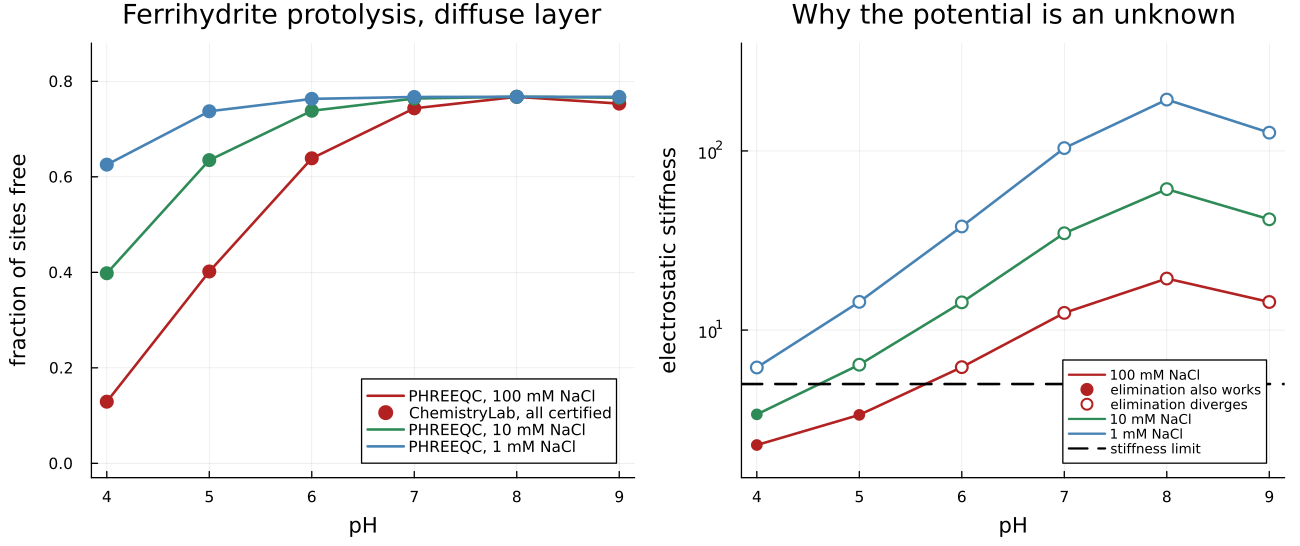
What this settles and what it does not
The Gouy-Chapman closure is implemented and matched against PHREEQC on every one of eighteen points, to 2.1 × 10⁻⁴ absolute on a site fraction, using this package's own Johnson-Norton dielectric constant — κ = 0.117215 against the
0.1174PHREEQC carries in its source. Adopting PHREEQC's makes the match very slightly worse, which rules the constant out as the cause of the residual and makes the agreement a stronger result: it holds with a different constant, not because of a shared one.The residual is not the aqueous activity model either, and three of them now say so: ideal gives 2.12 × 10⁻⁴ absolute, Davies 2.07 × 10⁻⁴ and SIT 2.09 × 10⁻⁴ — two per cent apart. Nor is it a missing surface complex: the weak-site block of
phreeqc.datdefines twenty-nineHfo_wspecies and a sodium chloride system can form three of them. What is left is small, and saying it is unattributed is worth more than naming a cause that measurement does not support.A diffuse-layer solve is a self-consistent speciation, not a certified minimum: the model's activity map is not the gradient of any Gibbs energy, and carrying the potential as an unknown does not change that. The theory page measures it, and separates it carefully from the constant capacitance, which is a gradient.
The published Dzombak & Morel metal calibration is now within reach: the acid-base half is reproduced at circumneutral pH, which is where the elimination used to stop. The metal half needs the zinc of the sorption edge run with the layer on, and that is the next step rather than a claim made here.
See also
Chemistry that happens on a surface — §9 derives the inversion and the two consistency criteria it separates.
Two families of sites, and a metal between them — the same oxide, with a metal, without electrostatics.
Surface areas — how a site family is declared.