Differentiating with respect to the parameters

Every constitutive law in this package is parameterised by the type of its coefficients — BBM{T}, never κ::Float64 — so a ForwardDiff.Dual can be placed in a material parameter, not only in the strain. This page is what that buys.

The distinction matters more than it looks. A solver that differentiates with respect to its unknowns gets a Jacobian and therefore Newton's method; that is table stakes, and VoronoiFVM and Ferrite already provide it. Differentiating with respect to the parameters answers a different class of question: which parameters does my experiment actually determine, how uncertain is a calibrated value, and which measurement would reduce that uncertainty. Those are the questions a soil laboratory asks, and they need derivatives that finite differences can only approximate — noisily, and at a cost that grows with the number of parameters.

The Barcelona Basic Model is the hard case, so it is the one used here. Its response goes through a return mapping — a Newton solve — and each step of a stress-controlled path goes through another. Derivatives have to survive both.

using PoroMechanics
using Tensors
using ForwardDiff
using LinearAlgebra
using Printf
using Random
using Plots

Sensitivities, and the zeros only automatic differentiation can see

A deviatoric path with a suction step, so that every parameter has a chance to matter.

reference = (κ = 0.011, λ0 = 0.065, r = 0.75, β = 2.0e-5, M = 1.2, k_s = 0.8, κ_s = 0.005, nu = 0.15)
parameter_names = collect(string.(keys(reference)))

function piecewise_linear(ts, fs, t)
    t <= first(ts) && return first(fs)
    t >= last(ts) && return last(fs)
    i = findlast(<=(t), ts)
    i == length(ts) && return last(fs)
    return fs[i] + (fs[i + 1] - fs[i]) * (t - ts[i]) / (ts[i + 1] - ts[i])
end

"Final state of a deviatoric, suction-stepped path, as a function of the eight parameters."
function deviatoric_path(θ; nstep = 200)
    m = BBM(
        κ = θ[1], λ0 = θ[2], r = θ[3], β = θ[4],
        M = θ[5], k_s = θ[6], κ_s = θ[7], nu = θ[8],
    )
    T = eltype(θ)
    st = initial_state(m, -1.0e3 * one(SymmetricTensor{2, 3, T}), T(4.0e4); suction = zero(T))
    Δt = 3.0 / nstep
    for k in 1:nstep
        t = k * Δt
        p = 1.0e3 * piecewise_linear([0, 1, 2, 3], [1, 40, 1, 80], t)
        q = 1.0e3 * piecewise_linear([0, 1, 2, 3], [0, 20, 1, 40], t)
        s = 1.0e3 * piecewise_linear([0, 1.999, 2, 3], [0, 0, 40, 40], t)
        σ = SymmetricTensor{2, 3, T}(
            (i, j) -> i != j ? zero(T) :
                i == 2 ? T(-(p + 2q / 3)) : T(-(p - q / 3))
        )
        _, _, st, _ = stress_controlled_response(m, σ, T(s), st, Δt)
    end
    return st
end

θ_ref = collect(values(reference))
observable(θ) = deviatoric_path(θ).εv_p

gradient_ad = ForwardDiff.gradient(observable, θ_ref)
gradient_fd = map(eachindex(θ_ref)) do i
    h = 1.0e-6 * abs(θ_ref[i])
    θp = copy(θ_ref); θp[i] += h
    θm = copy(θ_ref); θm[i] -= h
    (observable(θp) - observable(θm)) / (2h)
end

println("∂εv_p/∂θ")
println("  parameter   automatic differentiation   central differences")
for i in eachindex(θ_ref)
    @printf("  %-10s  %+.10e          %+.10e\n", parameter_names[i], gradient_ad[i], gradient_fd[i])
end

∂εv_p/∂θ
  parameter   automatic differentiation   central differences
  κ           -6.0737925136e-01          -6.0737925201e-01
  λ0          +3.8062668251e-01          +3.8062668255e-01
  r           +5.8955667903e-02          +5.8955667903e-02
  β           -4.8105833541e+02          -4.8105833483e+02
  M           -6.2099194573e-03          -6.2099194594e-03
  k_s         -1.3282771584e-03          -1.3282771454e-03
  κ_s         -7.1435018823e-18          -6.9388939039e-10
  nu          +1.7662441805e-13          +0.0000000000e+00

Six of the eight agree to nine or ten digits. The other two are the interesting ones.

and come back as and from automatic differentiation, and as from finite differences. Automatic differentiation is right and the finite differences are noise: the path is prescribed in stress, and under stress control the plastic strain is fixed by the yield surface and the hardening law alone. The elastic constants decide what strain accompanies that stress, not how much of it is plastic. The derivative is therefore structurally, exactly zero.

That is not a curiosity. A calibration that fits and tries to determine from it is fitting nothing, and a finite-difference gradient will hide that behind a small non-zero number rather than reporting it.

Which parameters can an experiment determine?

The usual identification experiment for the loading–collapse curve is isotropic compression repeated at several suctions. Four parameters shape it: and set the elastic and virgin compression lines, and and set how falls with suction,

Whether a given choice of suction levels determines all four is a question about the rank of — a matrix this package can produce exactly.

Parameters are scaled by their reference values, so the Jacobian is dimensionless and its condition number means something. Without that, comparing a sensitivity to   with one to   would be comparing units.

identification_names = ["κ", "λ(0)", "r", "β"]
θ_lc = [reference.κ, reference.λ0, reference.r, reference.β]

"Isotropic compression at a sequence of suctions; returns the measured volumetric strains."
function compression_protocol(θ, legs; nsub = 30, every = 6)
    m = BBM(κ = θ[1] * θ_lc[1], λ0 = θ[2] * θ_lc[2], r = θ[3] * θ_lc[3], β = θ[4] * θ_lc[4])
    T = eltype(θ)
    I3 = one(SymmetricTensor{2, 3, T})
    st = initial_state(m, -1.0e3 * I3, T(4.0e4); suction = zero(T))
    measurements = T[]
    p_now, s_now = 1.0e3, 0.0
    for (s, p_max, p_min) in legs
        for k in 1:15                                   # change the suction at constant stress
            _, _, st, _ = stress_controlled_response(
                m, -p_now * I3, T(s_now + (s - s_now) * k / 15), st, 1.0
            )
        end
        s_now = s
        for (a, b) in ((p_now, p_max), (p_max, p_min))  # load, then unload
            for k in 1:nsub
                _, _, st, _ = stress_controlled_response(
                    m, -(a + (b - a) * k / nsub) * I3, T(s), st, 1.0
                )
                k % every == 0 && push!(measurements, tr(st.ε))
            end
        end
        p_now = p_min
    end
    return measurements
end

plausible = [(0.0, 100.0e3, 10.0e3), (100.0e3, 200.0e3, 10.0e3), (300.0e3, 300.0e3, 10.0e3)]
informative = [(0.0, 80.0e3, 20.0e3), (50.0e3, 200.0e3, 20.0e3), (150.0e3, 400.0e3, 20.0e3)]

function report_design(label, legs)
    J = ForwardDiff.jacobian(θ -> compression_protocol(θ, legs), ones(4))
    F = svd(J)
    @printf("%s\n  singular values: %s\n", label, join([@sprintf("%.2e", x) for x in F.S], "  "))
    @printf(
        "  weakest direction: %s\n\n", join(
            [@sprintf("%s %+.2f", identification_names[i], F.V[i, end]) for i in 1:4], "   "
        )
    )
    return F
end

svd_plausible = report_design("Suctions 0, 100, 300 kPa — a plausible choice", plausible)
svd_informative = report_design("Suctions 0, 50, 150 kPa", informative)

LinearAlgebra.SVD{Float64, Float64, Matrix{Float64}, Vector{Float64}}
U factor:
30×4 Matrix{Float64}:
 -0.0109983   0.122542    0.389149    0.0647205
 -0.0135826   0.151336    0.480587    0.0799278
 -0.0244275   0.195146    0.361067    0.0254921
 -0.0396297   0.247798    0.136291   -0.0642643
 -0.0514464   0.288738   -0.0383361  -0.13401
 -0.0508128   0.281679   -0.0607521  -0.137738
 -0.050056    0.273246   -0.0875318  -0.142192
 -0.0491159   0.262771   -0.120795   -0.147724
 -0.0478745   0.24894    -0.164719   -0.155029
 -0.0460423   0.228526   -0.229546   -0.165811
  ⋮                                  
 -0.191416    0.0867351  -0.0179154   0.244037
 -0.192842    0.102629    0.0325575   0.252431
 -0.283178   -0.0925903   0.252181   -0.129048
 -0.304003   -0.0923335   0.169979   -0.168623
 -0.303181   -0.101486    0.140915   -0.173457
 -0.302139   -0.113096    0.104044   -0.179589
 -0.300713   -0.12899     0.0535715  -0.187983
 -0.298439   -0.154318   -0.0268612  -0.20136
 -0.292325   -0.222449   -0.243218   -0.237343
singular values:
4-element Vector{Float64}:
 0.488018611860158
 0.13061276836737368
 0.04099704288003035
 0.023289715531069743
Vt factor:
4×4 Matrix{Float64}:
  0.230594    0.536144   0.808081   -0.0798882
 -0.687633   -0.497386   0.528452    0.0224955
 -0.685415    0.665109  -0.259796   -0.142629
 -0.0647576   0.150954   0.0158308   0.98629

The first protocol looks entirely reasonable and cannot determine at all: the smallest singular value is , and the direction it belongs to is alone. Two things conspire, and neither is visible from the protocol itself.

At   kPa the sample never reaches its yield surface — the preconsolidation pressure the loading–collapse curve puts there, about 225 kPa, is beyond the 200 kPa the leg applies — so that leg carries no information about whatever. And at   kPa,  , so has already collapsed to zero and has saturated at  , with no longer in it. The one leg that does yield is the one where has stopped mattering.

The second protocol puts the suctions where is of order one — 0, 1 and 3 — and raises each leg's peak pressure past the yield surface that the previous leg left behind. All four singular values are then healthy, spanning a factor of about twenty.

This is the practical payoff, and it comes before any experiment is run: the parameters are not a property of the model alone but of the model and the measurement, and a Jacobian says which is which. A finite-difference version of this calculation costs five forward simulations instead of one and returns singular values contaminated by step-size error — precisely where the small ones, the ones that matter, live.

Calibration

Synthetic measurements from the informative protocol, with 10⁻⁴ of measurement noise on a strain of order 10⁻¹ — about what a volumetric strain measurement achieves.

Random.seed!(20260827)
truth = ones(4)
measurements = compression_protocol(truth, informative) .+ 1.0e-4 .* randn(30)
residual(θ) = compression_protocol(θ, informative) .- measurements

residual (generic function with 1 method)

Levenberg–Marquardt, with the Jacobian from ForwardDiff rather than from differences. The damping is what makes it robust to a poor starting point; the exact Jacobian is what makes the steps near the solution good ones.

function levenberg_marquardt(f, θ; λ = 1.0e-3, maxiter = 40)
    r = f(θ)
    cost = sum(abs2, r)
    history = [cost]
    for _ in 1:maxiter
        J = ForwardDiff.jacobian(f, θ)
        H = J' * J
        g = J' * r
        improved = false
        for _ in 1:30
            δ = -(H + λ * Diagonal(diag(H))) \ g
            θ_new = θ .+ δ
            r_new = f(θ_new)
            cost_new = sum(abs2, r_new)
            if cost_new < cost
                θ, r, cost = θ_new, r_new, cost_new
                λ = max(λ / 3, 1.0e-12)
                improved = true
                break
            end
            λ *= 5
        end
        push!(history, cost)
        improved || break
        length(history) > 2 && abs(history[end - 1] - history[end]) < 1.0e-16 * history[end] &&
            break
    end
    return θ, history, r
end

θ_start = [1.35, 0.80, 1.15, 0.65]        # 35 %, 20 %, 15 %, 35 % away
θ_fit, history, residual_final = levenberg_marquardt(residual, copy(θ_start))

@printf("Levenberg–Marquardt: %d iterations, cost %.3e → %.3e\n\n", length(history) - 1, first(history), last(history))

Levenberg–Marquardt: 9 iterations, cost 2.313e-03 → 2.964e-07

The covariance of the fitted parameters follows from the same Jacobian,   with the residual variance. It is available only because the derivatives are.

J_fit = ForwardDiff.jacobian(residual, θ_fit)
σ² = sum(abs2, residual_final) / (length(measurements) - length(θ_fit))
# The normal matrix is symmetric by construction, and saying so is not cosmetic: formed as
# a plain product it comes back asymmetric in the last bits, and an inverse that inherits
# that is no longer a covariance — it fails a positive-definiteness check for a reason that
# has nothing to do with the experiment.
Σ = σ² * inv(Symmetric(J_fit' * J_fit))

println("parameter    true         start        identified   standard error")
for i in eachindex(θ_fit)
    v = θ_lc[i]
    @printf(
        "  %-8s   %-11.5g  %-11.5g  %-11.5g  ± %.2g\n",
        identification_names[i], v, θ_start[i] * v, θ_fit[i] * v, sqrt(Σ[i, i]) * v
    )
end

parameter    true         start        identified   standard error
  κ          0.011        0.01485      0.010983     ± 2.1e-05
  λ(0)       0.065        0.052        0.0652       ± 0.00012
  r          0.75         0.8625       0.74876      ± 0.00062
  β          2e-05        1.3e-05      1.9975e-05   ± 9e-08

All four are recovered to a few parts in a thousand from a start more than a third away, in nine iterations.

The sensitivity figure

What the calibration is exploiting, drawn: how each measurement in the protocol responds to each parameter. Flat curves are parameters the experiment cannot see.

J_plot = ForwardDiff.jacobian(θ -> compression_protocol(θ, informative), ones(4))
plt = plot(
    1:size(J_plot, 1), J_plot;
    label = reshape(["∂εv/∂ln " .* identification_names...], 1, :),
    xlabel = "measurement number along the protocol",
    ylabel = "relative sensitivity",
    lw = 2, legend = :bottomleft, size = (760, 420),
)
vline!(plt, [10.5, 20.5]; ls = :dash, c = :gray, label = "suction step")
plt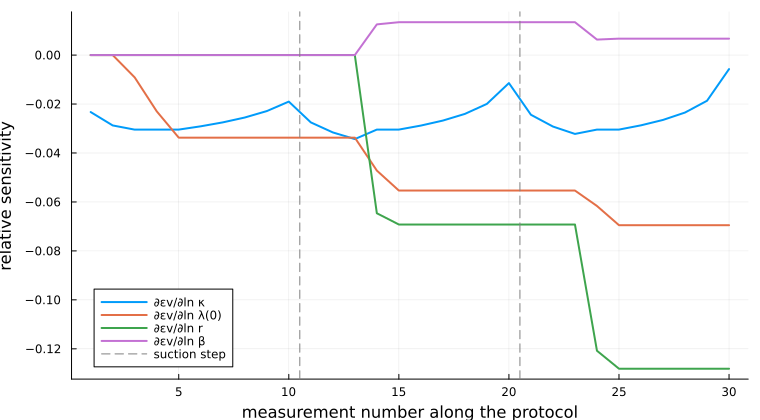

The three groups of ten are the three suction levels. and are felt everywhere, growing as the sample is compressed further. and do nothing at all in the first group — at zero suction   whatever they are — and only separate from each other across the second and third. That is the picture behind the rank deficiency of the first protocol, and the reason the third suction level is not optional.