Biot consolidation: water and deformation in a dam

Imagine squeezing a water-filled sponge. Its solid skeleton deforms, the water pressure changes, and water flows if it can escape. Concrete and rock behave much more stiffly, but the same interaction is the subject of Biot poroelasticity. Here we apply it to a two-dimensional section of the Ternay dam and its foundation when a reservoir load is applied suddenly.

This tutorial assumes basic calculus, matrix algebra, and Hooke's law. We will connect the physical picture to conservation equations, then follow their finite element implementation with PoroMechanics and Ferrite. It is an illustrative linear model, not a complete assessment of the real dam's safety.

1. What are we calculating?

There are three scalar unknowns at each mesh node:

Unknown	Meaning	Unit
	Horizontal displacement; positive to the right	m
	Vertical displacement; positive upward	m
	Liquid pore pressure relative to the reference pressure	Pa

The displacement vector is  . Pressure acts inside the pores; it is distinct from the external water force on the upstream surface. The model accounts for both effects.

The pores stay saturated throughout the calculation. A pressure of zero means the reference pressure, not the absence of water. In particular, this example does not simulate a wetting front entering an initially dry dam. Unlike the drying tutorial, it has neither a gas phase nor temperature as an unknown.

Geometry and boundary conditions

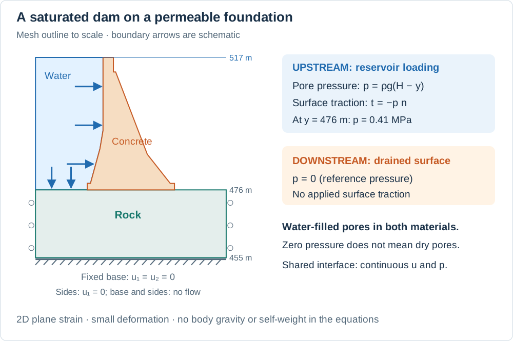
The outline follows the supplied mesh. Arrows illustrate boundary conditions, not computed displacements or velocities; the reservoir is outside the mesh.

The file ternay.msh contains 479 nodes and 860 triangular cells, with two material regions: concrete (physical surface "1") and rock ("2"). Coordinates are in meters. The water surface is at elevation   m and the dam-foundation interface is at   m. The reservoir imposes

Using    Pa/m, the upstream pressure increases from zero at the water surface to   Pa, or MPa, at the interface. The outward unit normal is : therefore an inward water force has traction   . Traction is force per unit area.

Mesh tags	Hydraulic condition	Mechanical condition
101–105, 121: upstream
106–112, 125: downstream	(drained boundary)	Zero applied traction
122, 124: foundation sides	Zero normal flow	; vertical sliding is allowed
123: foundation base	Zero normal flow

A prescribed value is a Dirichlet condition. Zero flow and zero traction on otherwise unconstrained boundaries are natural conditions of the weak form introduced below. A shared mesh joins concrete and rock: displacement and pressure are continuous across their interface, while the assembly enforces force and flux balance in the weak sense. No contact opening or interface leakage law is added.

Assumptions and initial state

We assume small strains, isotropic linear elasticity, saturated pores, constant material coefficients, and slow enough loading to neglect inertia. The section is in plane strain: out-of-plane strain is zero, not out-of-plane stress. All integrals represent a section with unit thickness perpendicular to the drawing. Cracking, plasticity, temperature changes, and dam self-weight are omitted.

Gravity is omitted from the bulk mechanical and Darcy equations. It appears only through the prescribed reservoir pressure. This distinction matters: the interior flow law below is driven by pressure gradients, not by a full hydraulic-head gradient including elevation. Do not interpret this example as a complete self-weight and gravitational seepage calculation.

The code starts with zero displacement and zero pressure at unconstrained nodes, and immediately imposes the upstream pressure at the boundary. It then applies the reservoir traction for the first time step. This represents a sudden load increment on an idealized reference state. The initial zero displacement is not an equilibrium solution under the newly applied traction; equilibrium is enforced at the first solved step.

2. From the physical picture to the equations

Compression can raise pore pressure; pressure changes the stress carried by the solid skeleton. Flow gradually redistributes the water. Both unknowns are solved together at every step.

Small strain and force balance

Displacement is a movement; strain measures how that movement varies in space:

Strain is dimensionless. For example, a bar lengthening by 1 mm over 1 m has axial strain . Positive volumetric strain denotes expansion; negative volumetric strain denotes compression.

With tension taken as positive, the total stress is

Here is the identity tensor and is the dimensionless Biot coefficient. The minus sign makes positive pore pressure contribute compressive stress. At fixed total load, changing changes the load supported by the skeleton, so the displacement changes too. The Lamé constants are calculated from Young's modulus and Poisson's ratio :

Do not confuse the shear modulus [Pa] with liquid viscosity [Pa·s]. Under plane strain,   but     generally is not zero.

Water storage and Darcy flow

Let denote the change in fluid content: the additional fluid mass, divided by the reference liquid density and the reference bulk volume. It is dimensionless: an equivalent fluid volume per initial bulk volume. Linear poroelasticity writes, with pressure measured from the reference state,

The first term describes storage associated with deformation. The second describes pressure-dependent storage at fixed strain. is a storage coefficient, in Pa⁻¹; it is the inverse of the Biot modulus often denoted in other texts. is the Darcy volume flux relative to the solid skeleton [m/s], not the velocity of an individual water molecule or the mass flux. Intrinsic permeability [m²] measures how easily the pore network transmits water.

As a sign check, consider a locally undrained compression: no water leaves, so  . Then   . A negative strain increment raises pressure. This simple calculation explains the coupling without assuming that every point in this dam follows an undrained path.

Conservation means “rate of accumulation + net outflow = zero”:

Both terms have units s⁻¹. This is the constant-reference-density fluid mass balance written in terms of fluid content. Together with force balance, it supplies three scalar equations for , , and .

Does the volume in the conservation law change?

Yes: the material deforms, but it is water mass that is conserved. Imagine a small piece of the dam whose boundary follows the solid skeleton. Call its current domain . Its volume can change, and water can cross its moving boundary. Without a fluid source, the exact integral balance is

Here is the current porosity, the current liquid density, and and the liquid and solid velocities. The integral on the left is the water mass inside the deforming piece; the one on the right is its outward mass flow rate. The derivative includes the motion of the domain, not just a change in at fixed coordinates. A boundary moving with the solid does not necessarily move with the water, which is why the flux uses the relative velocity.

To express this balance on an unchanged reference domain , introduce the local volume ratio  . The water mass per reference bulk volume is , and the dimensionless change in fluid content is

Subscript 0 denotes the reference state, where  . Dividing by the fixed reference density is a choice of units; it does not require the actual liquid to be incompressible. Notice that both changing pore volume and changing liquid density can change the amount of water stored.

In small-strain theory,   . Linearizing the storage law gives   . Consistently linearizing the balance and flux about the reference state gives

Dots denote time derivatives following the reference material points. Thus the fixed mesh used by this example does not assume a constant physical volume: its first-order effect is retained through . At finite deformation, one would need the full volume ratio and transformations of areas and fluxes between current and reference configurations. Those geometric effects are outside this linear example.

Must the material be free to deform?

No. The mass balance holds whether displacement is allowed or constrained. Small deformation, rather than unrestricted deformation, is the assumption behind its linear form. Mechanical conditions determine which strain occurs; hydraulic conditions determine how water can enter or leave.

Situation	Consequence for the local balance	Interpretation
Locally fixed volume:		Pressure-dependent storage remains even without bulk-volume change.
Locally undrained compression:		Water mass stays constant while compression raises pressure.

For the first case, compressibility allows fluid exchange to change pressure even though the bulk volume is fixed. For the second, imagine a sealed, uniformly compressed small specimen. Sealing the exterior of a large heterogeneous domain fixes its total water mass but does not prevent internal redistribution: it does not by itself imply   at every point.

Our dam already has mechanical constraints: the foundation base is fixed and its sides cannot move horizontally. These conditions do not set volumetric strain to zero everywhere. Likewise, a drained boundary does not imply a mechanically free boundary. Keep the two types of conditions separate when interpreting the model.

Parameters and a useful time-scale estimate

Symbol	Concrete	Rock	Unit	Meaning
			Pa	Elastic stiffness
	0.15	0.15	—	Lateral strain response
			m²	Intrinsic permeability
	0.4	0.2	—	Pressure–deformation coupling
			Pa⁻¹	Storage coefficient at fixed strain
			Pa·s	Liquid viscosity

The coefficient of consolidation is not the effective storage. To see the distinction, consider a separate, homogeneous one-dimensional column, with deformation along , lateral strains held at zero, and axial total stress held constant after a load increment. Its axial strain is its volumetric strain, and the axial constitutive equation gives

The column is laterally constrained but can shorten in the axial direction. Substituting this relation into the water balance, with constant coefficients, yields a pressure diffusion equation:

Quantity	Unit	Physical role
	Pa⁻¹	Storage response to pressure at fixed strain
	Pa⁻¹	Storage response including the strain allowed by this column's mechanical conditions
	m²/s	Diffusivity governing the redistribution of pressure

The extra term   is the mechanical contribution to effective storage. It follows from the stated column constraints; it is not a universal replacement for under any mechanical boundary conditions. The dam solver retains displacement and pressure as coupled unknowns and does not substitute this scalar estimate for their equations.

Consolidation connects this diffusion to deformation. A rapid compressive load on a saturated specimen can first raise pore pressure. As water drains, the excess pressure dissipates, the skeleton carries more of the fixed total load, and the specimen progressively compresses. This delayed deformation associated with drainage is consolidation. Larger permeability speeds up the process; larger effective storage slows it down for a given permeability and viscosity.

Balancing the time and space derivatives in the diffusion equation gives the characteristic time for a drainage length :

This is a time-scale estimate, not an exact time to complete consolidation; numerical factors depend on the boundary conditions and chosen degree of consolidation. Dissipation refers to excess pressure relative to the eventual steady state, whose pressure need not be zero. In the dam example, hydraulic boundary loading also acts alongside the mechanical reservoir force.

The material values here give   m²/s for concrete and m²/s for rock. For an illustrative drainage length   m, the corresponding times are about 1,108 s (18.5 min) and 1.02 s. Doubling multiplies the estimate by four. These estimates explain why rock responds faster; they are not an analytical solution or a completion time for this heterogeneous two-dimensional dam.

The default simulation lasts     s, or 33.3 min. A 100 s step cannot resolve a process occurring in approximately one second. Implicit integration can remain stable with that step while missing the fast initial rock response.

3. How to run the example

From the repository root, prepare the examples environment once:

julia --project=examples -e 'using Pkg; Pkg.develop(path="."); Pkg.instantiate()'
julia --project=examples examples/biot_consolidation/run.jl

Use Julia 1.12 or newer. The script needs Ferrite, FerriteGmsh, and the supplied ternay.msh; run it in the examples environment, which declares these dependencies. The mesh path is relative to this script, so it does not depend on the working directory. The documentation displays this example without executing it during its build; run the command above to perform the calculation yourself.

PoroMechanics supplies the Biot assembly and time integration. This example defines the reservoir traction through facet_load!; Ferrite manages shape functions, quadrature, degrees of freedom, constraints, and assembly. There is no VoronoiFVM flux! or nonlinear Newton iteration in this linear example.

using PoroMechanics
using Ferrite
using FerriteGmsh
using LinearAlgebra
using Printf

4. Define the model and the result

BiotModel <: AbstractPoroModel groups the material data and reservoir loading. concrete and rock are reusable BiotPoroelastic materials. The FEM field :u has two components and :p has one. nspecies and species_names describe these three scalar components in the PoroMechanics interface.

The parameter rho_g = rho_l * g is the product of liquid density and gravitational acceleration, expressed in Pa/m. The load uses rho_g directly. Each material carries its fluid viscosity mu_l; the loading carries rho_g. If you change the fluid, update both viscosities and rho_g consistently.

BiotSolution holds the final solution vector and its DofHandler. The latter is the map between physical fields, mesh nodes, and positions in the vector; guessing that all pressures occupy the last third of the vector is unsafe.

"""Parameters of model M7 (Biot poroelasticity, saturated medium)."""
Base.@kwdef struct BiotModel{C, R, T, G} <: AbstractPoroModel
    concrete::C = BiotPoroelastic(;   # surface "1"
        E = 1.4e10, nu = 0.15, k = 1.0e-14, b = 0.4, N = 1.0e-10, mu_l = 1.0e-3,
    )
    rock::R = BiotPoroelastic(;       # surface "2"
        E = 1.8e10, nu = 0.15, k = 1.0e-11, b = 0.2, N = 1.0e-10, mu_l = 1.0e-3,
    )
    H::T = 517.0                    # water table elevation [m NGF]
    rho_g::G = 10_000.0              # liquid density × gravity [Pa/m]
end

PoroMechanics.nspecies(::BiotModel) = 3   # u₁, u₂, p
PoroMechanics.species_names(::BiotModel) = [:u1, :u2, :p]

"""Result of the M7 simulation: solution vector and DofHandler."""
struct BiotSolution
    x  :: Vector{Float64}
    dh :: DofHandler
end

function Base.show(io::IO, r::BiotSolution)
    print(io, "BiotSolution: $(length(r.x)) DOFs — reach them through .x and .dh")
end

"Hydrostatic reservoir pressure at elevation y [Pa]."
p_hydro(m::BiotModel, y::Real) = m.rho_g * (m.H - y)

5. From differential equations to element matrices

Why use a weak form?

The strong equations require force and water balances at each point. They contain spatial derivatives of stress and flux, which themselves depend on derivatives of displacement and pressure. However, the continuous, piecewise-linear fields used on our triangles have gradients that can jump between cells. Their classical second derivatives are not defined everywhere.

The weak formulation transfers one spatial derivative to a test function by integration by parts. It uses only first derivatives of the unknowns, and boundary forces and fluxes appear explicitly. Here is the fixed reference domain of the small-strain model discussed above.

Before discretization, requiring the weak equations for every admissible test function is a reformulation of the balance laws, with lower smoothness requirements. It does not mean that conservation is optional or approximate. The finite element approximation comes later, when we restrict unknowns and tests to finite-dimensional spaces. It does not automatically enforce an exact local balance on every cell.

Step 1: choose admissible test functions

Let be a vector test function for displacement and a scalar test function for pressure. A test function weights the residual of an equation; requiring every such weighted integral to vanish expresses the balance throughout the domain. Mechanically, can also be interpreted as a virtual displacement. It is not the solid velocity and is not an additional unknown.

Why must the tests vanish on prescribed-value boundaries? Suppose that   is imposed there. A trial variation   must keep that value for any small scalar , so the corresponding components of must be zero. Similarly,   requires  . The prescribed values themselves need not be zero.

Field	Essential (Dirichlet) boundary	Natural boundary
Displacement	Prescribe ; set the corresponding components of to zero	Prescribe traction
Pressure	Prescribe on ; set   there	Prescribe outward flux    on

For displacement, the split is componentwise: on the foundation sides,   implies  , while is unrestricted and the vertical traction is zero. At the fixed base, both test components vanish. Reactions at constrained components are not prescribed tractions; they are determined by the solution.

Step 2: integrate mechanical equilibrium by parts

There is no body force in this example. Multiply    by and integrate:

Recall the one-dimensional identity   . The divergence theorem gives its multidimensional counterpart:

The boundary normal points outward. The colon is a tensor dot product:   . Since stress is symmetric, its contraction with the antisymmetric part of is zero. Therefore    . Moving the volume term to the other side gives the virtual-work identity

Now insert    , where is the elastic stiffness tensor encoded by and . The identity     explains the pressure coupling term. Tests vanish at prescribed displacement components; the other boundary components contribute prescribed traction. Thus

Here the traction integral includes only unconstrained displacement components. It is the internal virtual work balanced by external virtual work. In the dam, the nonzero prescribed traction is    on the upstream boundary. facet_load! evaluates this right-hand side. The minus sign in the pressure coupling comes from the stress law, not from the choice of outward normal.

Step 3: integrate the water balance by parts

Start with storage plus net outflow:

A dot denotes a time derivative. Multiply by the pressure test , integrate, and apply integration by parts only to the flux divergence:

Substituting Darcy's law makes the interior transport term positive:     . The storage term already contains at most first spatial derivatives, so there is no need to integrate it by parts. On ,  ; on , the prescribed flux remains:

The sign convention matters:   denotes water leaving the body, so it contributes negatively to the right-hand side. An imposed inflow has the opposite sign. In this example the base and foundation sides have zero normal flux, so   and the hydraulic right-hand side vanishes.

A zero test function on a prescribed-pressure boundary does not mean zero flow there. Upstream and downstream water exchange is determined by the solution. Its boundary integral vanishes in this weak equation because   there, not because the physical flux is zero. The prescribed pressure values still enter the solution through the Dirichlet constraints.

Step 4: connect boundary terms and material interfaces to the code

ConstraintHandler imposes the essential conditions on :u and :p. facet_load! assembles the nonzero natural mechanical load. No hydraulic boundary load vector is needed for this example's zero prescribed fluxes. Omitting a boundary load on an unconstrained component implements the corresponding zero natural condition; it does not impose a zero field value.

The same integration by parts can be performed separately in concrete and rock. Their shared interface has opposite outward normals on its two sides. With no interface source or applied interface force, continuity of normal flux and traction makes the paired boundary terms cancel for continuous tests. This is why we assemble both materials on one shared mesh, using each cell's own coefficients. We do not differentiate permeability across its jump as if it were a smooth function.

The mechanical pressure term is negative,  ; the deformation-storage term is positive,  . These are the origins of the opposite coupling signs in the matrices below.

One triangle, nine degrees of freedom

“P1” means a polynomial of degree one: each field varies linearly over a triangle. There are three nodal pressure values and two displacement components at each of three nodes:     local degrees of freedom. Neighboring cells share nodal values. With 479 nodes, this gives 1,437 global degrees of freedom before constraints are imposed.

Write the vector displacement shape functions as and scalar pressure shape functions as . Approximate the fields by

In the Galerkin method, choose each basis function in turn as a test:   for the mechanical rows and   for the hydraulic rows, with the prescribed-value constraints accounted for. Substitution into the two weak equations gives a finite system for the nodal coefficients and . For example, the diffusion integral becomes   : the integral is a matrix entry, and is an unknown coefficient. The four element blocks are

Their sizes are respectively  ,  ,  , and  . Ferrite evaluates these integrals by quadrature, a weighted sum at points inside each cell. shape_value returns a basis function's value, shape_gradient its spatial gradient, and getdetJdV the geometric integration weight. reinit! updates these quantities for the current cell.

The implementation stores two matrices, with local unknown order :

Thus   : mechanics has no inertial or time-derivative term, whereas fluid content changes with both displacement and pressure. The opposite coupling signs follow directly from stress and storage; they are not arbitrary. The package function biot_element_matrices! implements these four blocks. assemble_biot_matrices calls it for each cell, using the material selected by material_at(cell). This example supplies that selector when assembling below.

6. Apply the reservoir force

The following callback integrates   over an upstream facet (an edge in two dimensions). getnormal supplies the outward normal, and spatial_coordinate supplies the elevation used for hydrostatic pressure. Pressure Dirichlet conditions will be added separately: imposing a pore pressure does not automatically apply a mechanical traction.

"""
    PoroMechanics.facet_load!(fe, facet, m::BiotModel, fv_u)

Adds the hydrostatic thrust  t = −p_hydro(y)·n  on the upstream face.
`fe` contains the six displacement entries associated with the adjacent P1 cell.
"""
function PoroMechanics.facet_load!(fe, facet, m::BiotModel, fv_u)
    coords = getcoordinates(facet)
    nu_l   = getnbasefunctions(fv_u)
    for q in 1:getnquadpoints(fv_u)
        x  = spatial_coordinate(fv_u, q, coords)
        n  = getnormal(fv_u, q)
        dΓ = getdetJdV(fv_u, q)
        t  = -p_hydro(m, x[2]) * n   # inward traction
        for i in 1:nu_l
            Nu = shape_value(fv_u, q, i)
            fe[i] += (Nu ⋅ t) * dΓ
        end
    end
end

7. Assemble and advance in time

The solver first reads the mesh and creates a DofHandler for :u and :p. A ConstraintHandler records prescribed values. Cell contributions are added to global sparse matrices through assemble!, using celldofs to find their positions. The matrices and are assembled once because the material laws and geometry are constant.

Backward Euler replaces at the new time by  . Rearranging gives the actual linear system in the code:

Its second block row is worth reading explicitly:

This is precisely “deformation storage + pressure storage + flow = zero”. apply!(A, rhs, ch) enforces the boundary values; A \ rhs solves the coupled system. There is one linear solve per time step, with no staggered iteration. The current implementation forms A and invokes its factorization at every step. Reusing a factorization for a fixed step and unchanged constraints would be a possible optimization; it is not implemented by solve_biot.

solve_biot applies initial boundary values, updates constraints at each supplied time, and calls report_step with the converged state. The callback below only prints case-specific diagnostics; it does not assemble or advance the solution.

Backward Euler is first-order accurate in time. Its robustness does not remove the need to check time-step and mesh sensitivity, particularly just after the sudden change in loading.

"""
    run_biot(; model = BiotModel(), dt, n_steps, mesh_path)

Simulates the consolidation of the Ternay dam by Biot poroelasticity (M7).

Returns `BiotSolution(x, dh)`: the solution vector at the last step and the DofHandler,
so that results can be post-processed later (extracting p or u per node).

# Keyword arguments
- `model`     : materials and reservoir loading (default: `BiotModel()`)
- `dt`        : time step [s] (default: 100 s)
- `n_steps`   : number of steps (default: 20 → t_max = 2000 s = 33.3 min)
- `mesh_path` : path to `ternay.msh` (default: the script's own directory)
"""
function run_biot(;
    model     = BiotModel(),
    dt        = 100.0,
    n_steps   = 20,
    mesh_path = joinpath(@__DIR__, "ternay.msh"),
)
    m = model

    # ── Mesh ─────────────────────────────────────────────────────────────────
    grid = togrid(mesh_path)
    @printf("Mesh: %d nodes, %d elements\n", getnnodes(grid), getncells(grid))

    concrete_cells = getcellset(grid, "1")   # concrete elements

    # ── DofHandler : P1 vector (u₁,u₂) + P1 scalar (p) ─────────────────
    ip_geo = Lagrange{RefTriangle, 1}()
    ip_u   = Lagrange{RefTriangle, 1}()^2
    ip_p   = Lagrange{RefTriangle, 1}()

    dh = DofHandler(grid)
    add!(dh, :u, ip_u)
    add!(dh, :p, ip_p)
    close!(dh)

    n_loc = ndofs_per_cell(dh)
    n_tot = ndofs(dh)
    @printf("DOFs: %d total (%d per element)\n", n_tot, n_loc)

    # ── Quadrature ───────────────────────────────────────────────────────────
    qr     = QuadratureRule{RefTriangle}(3)
    qr_fac = FacetQuadratureRule{RefTriangle}(2)

    cv_u = CellValues(qr, ip_u, ip_geo)
    cv_p = CellValues(qr, ip_p, ip_geo)
    fv_u = FacetValues(qr_fac, ip_u, ip_geo)

    # ── Dirichlet conditions ──────────────────────────────────────────────────
    ch = ConstraintHandler(dh)

    upstream_tags   = ["101","102","103","104","105","121"]
    downstream_tags = ["106","107","108","109","110","111","112","125"]

    upstream_hyd   = reduce(union, getfacetset(grid, r) for r in upstream_tags)
    downstream_hyd = reduce(union, getfacetset(grid, r) for r in downstream_tags)

    add!(ch, Dirichlet(:p, upstream_hyd,   (x, t) -> p_hydro(m, x[2])))
    add!(ch, Dirichlet(:p, downstream_hyd, (x, t) -> 0.0))

    for reg in ["122","123","124"]
        add!(ch, Dirichlet(:u, getfacetset(grid, reg), (x, t) -> 0.0, [1]))
    end
    add!(ch, Dirichlet(:u, getfacetset(grid, "123"), (x, t) -> 0.0, [2]))

    close!(ch)
    update!(ch, 0.0)
    @printf("Contraintes Dirichlet : %d DDL prescrits\n", length(ch.prescribed_dofs))

    # ── Assemble the constant matrices and reservoir load ────────────────────
    material_at(cell) = cellid(cell) ∈ concrete_cells ? m.concrete : m.rock
    K1, K2 = assemble_biot_matrices(dh, cv_u, cv_p, material_at; constraints = ch)
    f_ext = assemble_biot_load(dh, upstream_hyd, fv_u, m)

    # ── Time loop — implicit Euler ────────────────────────────────────────────
    println("\nM7 Biot 2D — Ternay dam  (Δt = $(dt) s, $(n_steps) steps)")
    println("─"^66)
    println("Step |     t [d] | p_max concrete [MPa] | u₁_max [mm] | u₂_max [mm]")
    println("─"^66)

    u_range = dof_range(dh, :u)
    p_range = dof_range(dh, :p)

    function report_step(x, t_step, step)
        p_concrete_max = -Inf
        for ci in concrete_cells
            d = celldofs(dh, ci)
            for k in p_range
                p_concrete_max = max(p_concrete_max, x[d[k]])
            end
        end

        u1_max = 0.0;  u2_max = 0.0
        for ci in 1:getncells(grid)
            d = celldofs(dh, ci)
            for k in 1:2:length(u_range)
                u1_max = max(u1_max, abs(x[d[u_range[k]]]))
            end
            for k in 2:2:length(u_range)
                u2_max = max(u2_max, abs(x[d[u_range[k]]]))
            end
        end

        @printf("%4d | %9.4f | %+17.4f | %+11.4f | %+11.4f\n",
                step, t_step/86400.0, p_concrete_max/1e6, u1_max*1e3, u2_max*1e3)
    end

    x = solve_biot(K1, K2, ch;
        inival = zeros(n_tot), times = dt .* (0:n_steps),
        load = f_ext, on_step = report_step,
    )

    println("─"^66)
    println("Simulation finished.")

    return BiotSolution(x, dh)
end

8. Run and interpret the result

The following line runs the default case and retains the last state.

result = run_biot()

The printed table reports time in days, maximum concrete pressure in MPa, and maximum absolute displacement components in mm, over both materials. These last two numbers are magnitudes, not signed displacements at one common location. The maximum pressure may lie on a prescribed boundary and therefore change very little even while the interior field evolves. It cannot by itself establish that consolidation has finished.

For an interactive session, start julia --project=examples from the repository root, then run:

include("examples/biot_consolidation/run.jl")  # also runs the default case
fine_time = run_biot(dt=50.0, n_steps=40)     # same final time: 2,000 s
longer = run_biot(dt=100.0, n_steps=200)      # longer duration: 20,000 s

Compare equal physical times when studying time-step accuracy. Doubling the number of steps without changing dt changes the duration, not the resolution. Only the final state is returned. To save a time history, store copy(x) in the report_step callback; the solver reuses its solution buffer.

Recover values at nodes

Do not reshape .x into three columns: the DofHandler controls the ordering. Use node_dof_maps from PoroMechanics instead. Each map contains the global index of a field component at each mesh node:

grid = result.dh.grid
p_dofs = node_dof_maps(result.dh, grid, :p).p
u1_dofs = node_dof_maps(result.dh, grid, (:u, 1)).u
u2_dofs = node_dof_maps(result.dh, grid, (:u, 2)).u
pressure_MPa = result.x[p_dofs] ./ 1e6
horizontal_mm = result.x[u1_dofs] .* 1e3
vertical_mm = result.x[u2_dofs] .* 1e3

Request the two components of :u separately, as above. The resulting arrays follow mesh-node order and can be used to plot pressure contours and signed displacement fields. For a first time-step comparison on this unchanged mesh:

maximum(abs.(fine_time.x[p_dofs] - result.x[p_dofs]))  # pressure difference [Pa]
maximum(abs.(fine_time.x[u1_dofs] - result.x[u1_dofs])) # displacement difference [m]

A single difference is not an error estimate against an exact solution. Repeat with a smaller step to look for a consistent trend, and compare displacement and pressure separately because their units differ.

What should we expect physically?

The reservoir pushes inward on the upstream face and supplies pressure to its pores. The much more permeable foundation redistributes pressure faster than the concrete. Water exchange and deformation influence one another during this transient. An interior point can show a more complicated response than monotonic pressure decay: both hydraulic boundary loading and mechanical loading are present.

At steady state the storage derivative vanishes and

Within each constant-permeability material this reduces to Laplace's equation; across the interface the different permeabilities must still be respected. The imposed upstream pressure persists, so the steady state generally has nonzero pore pressure and continuing seepage. “Consolidated” does not mean “all pore pressures are zero”. The displacement is the equilibrium response to the external loading and that remaining pressure field.

9. Numerical limitations and checks

This is an equal-order P1/P1 mixed discretization without an added pressure stabilization term. Positive storage helps regularize the pressure equations, but does not guarantee freedom from spurious pressure oscillations. Small time steps, low permeability, and nearly incompressible or undrained limits can expose mixed-element stability problems. Ferrite's mixed elasticity tutorial explains the related inf-sup issue and the role of interpolation spaces; its pressure variable is an elastic constraint variable, whereas ours is pore pressure.

A completed linear solve or a passing regression test is not a convergence study. Before interpreting a changed parameter set quantitatively:

1. Refine the time step at a fixed final time; inspect the early response as well as the final state. The default step under-resolves the fast rock time scale.

2. Refine the mesh while preserving physical tags. Inspect pressure profiles near the interface and drained faces for alternating nodal oscillations. A smaller step alone does not fix a spatial stability problem.

3. Check prescribed values and supports. Verify the balance between fluid-content change and boundary outflow, and between applied forces and support reactions, with suitable post-processing. These balance diagnostics are not printed by the current script. Residual rows at prescribed pressure nodes represent boundary exchange and should not be interpreted as zero-flux conditions.

4. Assess the modeling assumptions before comparing with measurements: this case has no self-weight initialization, gravitational body-flow term, cracking, unsaturated flow, or site-specific parameter calibration.

The regression suite checks reproducibility against a stored solution. Run it from the repository root with julia --project -e 'using Pkg; Pkg.test(test_args=["regression"])'. It complements, rather than establishes, physical validation and discretization convergence. MOOSE's poroelasticity verification examples provide additional examples of checking storage and deformation against analytical solutions, using the alternative notation for our .

10. Short exercises

• Pressure and units: compute the upstream pressure at   m. You should obtain   Pa = MPa. Explain why the applied traction points inward.

• Coupling sign: for concrete, take an undrained volumetric strain increment of . Using the local storage relation gives    Pa. Explain why this is an illustrative local calculation, not a predicted dam profile.

• Constraints and drainage: can a specimen have fixed bulk volume while still exchanging water? Write the reduced mass balance and identify the storage term that remains. Does fixing the base of a dam impose that condition everywhere?

• Storage versus diffusivity: check the units of and . At fixed permeability, viscosity, and drainage length, what happens to and if the effective storage doubles?

• Drainage length: use   m in the time-scale estimate. Why is the estimate four times larger than at 10 m even though material coefficients are unchanged?

• Time resolution: compare 100 s, 50 s, and 25 s steps, all ending at 2,000 s. Examine pressure and displacement separately, including profiles rather than only the printed maxima.

• Permeability: supply a different concrete material without redefining the model:

  concrete = BiotPoroelastic(;
      E = 1.4e10, nu = 0.15, k = 1.0e-13, b = 0.4, N = 1.0e-10, mu_l = 1.0e-3,
  )
  more_permeable = run_biot(model = BiotModel(; concrete))

  This tenfold increase divides the homogeneous concrete time-scale estimate by ten; the coupled dam response still depends on geometry and on the foundation.

The two illustrations can be regenerated with python3 examples/biot_consolidation/draw_schematics.py. They describe geometry and coupling, not numerical results.