Getting Started

This page follows one simulation all the way through: from a sketch of the physical problem, to its equation, to the pieces a finite volume solver needs, to the Julia code that supplies those pieces, and finally to a plot of the result. The problem is deliberately simple, a tracer diffusing through a saturated porous medium. The steps, however, are the same for every finite volume model in the package, including the ones with several coupled unknowns.

The five steps

1. Describe the problem: the geometry, the unknown, and the boundary and initial conditions.

2. Write the equation as a balance: accumulation + net outflow = 0.

3. See what the solver asks for: the stored amount at a node, the flux between two neighboring nodes, and the boundary conditions.

4. Write those pieces as methods of a model type.

5. Build a grid, set the initial state, solve, and look at the result.

The package already ships this equation as FickModel, with per-region coefficients and its boundary data stored in a field. The page writes it again from scratch because what matters here is the mechanism, not the equation. It is called TracerModel so that the two names do not collide.

1. The problem to simulate

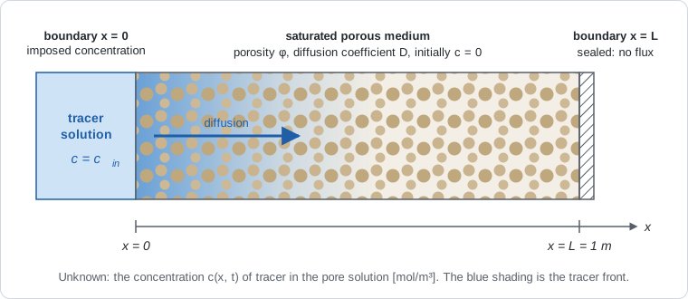
A slab of saturated porous medium, one meter long, initially contains no tracer. At   its left face is put in contact with a solution of concentration . The tracer enters the pore solution and diffuses to the right. The right face is sealed, so no tracer can leave through it.

The slab is uniform across its section, so nothing changes in or . The problem is therefore one-dimensional, with a single unknown: the concentration of tracer in the pore solution, in mol per m³ of solution.

Symbol	Value	Unit	Meaning
		—	porosity: volume fraction of the medium filled by the pore solution
		m²/s	effective diffusion coefficient of the tracer
		mol/m³	concentration imposed at
		m	length of the slab
		s	simulated duration, about three years

Where	Condition	Type
everywhere, at		initial condition
		Dirichlet: the value is imposed
	no flux through the face	homogeneous Neumann: the flux is imposed, equal to zero

2. The equation, read as a balance

Tracer is neither created nor destroyed. In any piece of the medium, the amount stored can therefore change only by what flows in or out:

The equation has two terms, and each one answers a separate question.

• The accumulation term answers how fast does the amount of tracer stored here change? It is built on the stored amount . is counted per m³ of pore solution, but only the fraction of the medium is solution, so is the amount of tracer per m³ of porous medium [mol/m³]. The accumulation term is its time derivative [mol/(m³·s)]: the rate at which that stored amount grows or shrinks. Keep the two apart. You will provide the stored amount, and the solver will take its time derivative.

• The flux answers how much tracer crosses a surface? It is an amount per unit area per unit time [mol/(m²·s)]. Fick's law says that tracer moves from high to low concentration, which is where the minus sign comes from. The factor is there because diffusion happens only through the pore solution.

• The divergence   is the net outflow per unit volume. When more tracer leaves a small volume than enters it, the stored amount decreases.

Substituting gives the more familiar form    . In one dimension:

The boundary conditions can be stated in the same terms:   at  , and   at  .

Why write the equation as a balance rather than as   ? Because the finite volume solver asks for exactly these two quantities, separately: the amount stored, and the flux. It handles the time derivative, the divergence and the rest by itself.

3. What the finite volume method does with it

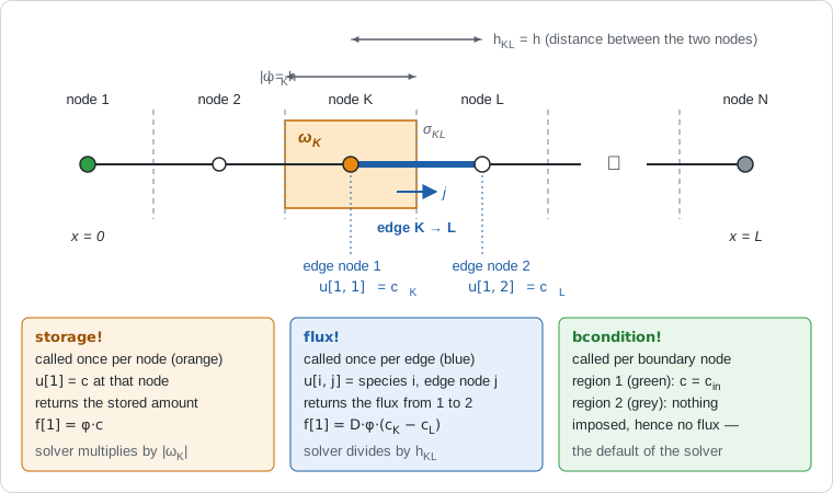
The grid places nodes along . Each node owns a control volume (orange), bounded by the midpoints between and its neighbors (dashed lines). Two neighboring nodes and are joined by an edge (blue), and their control volumes touch at an interface .

The balance of section 2 is then written for each control volume. Integrate it over and replace the time derivative by a difference over one time step (implicit Euler, where is the current step):

with

is the stored amount. comes from the flux through the interface: along the edge,       , and is the numerator of that expression. It is positive when tracer goes from to . In one dimension,   ( at the two end nodes),   (the interface is a point, counted per unit cross-section), and  .

This splits the work in two:

Piece of the discrete balance	In this problem	Provided by
stored amount		you: storage!
flux between two neighboring nodes		you: flux!
boundary conditions	at	you: bcondition!
number and names of unknowns	one unknown,	you: nspecies, species_names
geometry , ,	from the grid	VoronoiFVM
time derivative, sum over neighbors, Jacobian, Newton iterations, step size	—	VoronoiFVM

Your functions never see a derivative, a mesh size or a loop. They describe the physics locally, at one node or on one edge. The solver calls them for every node and every edge and puts the results together.

4. Writing the model

4.1 The parameters: a struct

using PoroMechanics
using VoronoiFVM
using ExtendableGrids

Base.@kwdef struct TracerModel <: AbstractPoroModel
    φ::Float64    = 0.30     # porosity [-]
    D::Float64    = 1e-10    # effective diffusion coefficient [m²/s]
    c_in::Float64 = 1.0      # concentration imposed at x = 0 [mol/m³]
end

TracerModel is a type. It states that a tracer model has a porosity, a diffusion coefficient and an inlet concentration; it does not fix their values. Base.@kwdef provides default values and a keyword constructor, so TracerModel() uses the defaults and TracerModel(D = 2e-10) changes only D. <: AbstractPoroModel declares the type as a model of this package, which is what fvm_system accepts.

4.2 Generic functions, and methods for your model

storage!, flux!, bcondition!, nspecies and species_names are generic functions that belong to PoroMechanics. In Julia, a generic function is a name that can carry several methods, and the method that runs is chosen from the types of the arguments. This mechanism is called multiple dispatch. The package declares these functions without knowing any particular model. Called on a model that has no method of its own, storage! stops with the error storage! not implemented for ….

When you write

PoroMechanics.storage!(f, u, node, m::TracerModel, data) = …

you add a method to that function. Julia uses it whenever the fourth argument is a TracerModel. Three consequences follow.

• The PoroMechanics. prefix is required. Without it, you would define a new, unrelated function called storage! in your own session, and the solver would never call it.

• The method is written for every TracerModel, not for one set of values. It reads m.φ and m.D when it runs. The numbers are supplied later, when you create an instance such as m = TracerModel() and pass it to fvm_system (section 5). The same method works unchanged for TracerModel(D = 1e-9).

• You never call these methods yourself. The solver calls them, for every node, every edge, every Newton iteration and every time step.

4.3 The anatomy of a callback

The three physics callbacks share the same argument list:

storage!(f, u, node, m, data)       # at one node
flux!(f, u, edge, m, data)          # on one edge
bcondition!(f, u, bnode, m, data)   # at one boundary node

Argument	What it is	Who fills it
f	the result: one entry per unknown, which you write into	you
u	the values of the unknowns where the callback is evaluated	the solver
node, edge, bnode	where the callback is evaluated: region number, coordinates, current time	the solver
m	your model, with its parameter values	fvm_system
data	a slot for user data in VoronoiFVM, unused here	the solver

The ! at the end of the name is the Julia convention for a function that modifies one of its arguments, here f. The value the function returns is ignored.

4.4 What u[1] and u[1, 1] mean

The shape of u depends on where the callback is evaluated.

• storage! and bcondition! look at a single node. There, u is a vector and u[i] is unknown number i at that node. With a single unknown, u[1] is the concentration at that node.

• flux! looks at an edge, which has two nodes. There, u is a matrix and u[i, j] is unknown number i at node j of the edge, with j = 1 or 2. So u[1, 1] is and u[1, 2] is (the blue labels in the figure above).

Expression	Callback	Meaning
u[1]	storage!, bcondition!	unknown 1 () at this node
u[1, 1]	flux!	unknown 1 () at the first node of the edge,
u[1, 2]	flux!	unknown 1 () at the second node of the edge,
u[2, 1]	flux!, model with two unknowns	unknown 2 at the first node of the edge

The first index counts unknowns, not nodes. In a model with two unknowns, for instance a liquid pressure and a temperature, u[2, 1] would be the temperature at the first node of the edge, and flux! would fill both f[1] and f[2], one flux per unknown.

"Node 1" and "node 2" here are local to the edge: its first end and its second end. They are not the nodes numbered 1 and 2 in the grid. The grid numbering only appears later, in the initial values (section 5.4).

4.5 storage!: the stored amount

function PoroMechanics.storage!(f, u, node, m::TracerModel, data)
    c = u[1]              # concentration at this node
    f[1] = m.φ * c        # stored amount s(c) = φ c
    return nothing
end

This is the stored amount  , the quantity inside . It is not the accumulation term itself. From it, the solver builds the accumulation term of the control volume: it computes   and multiplies it by . Returning a time derivative from storage! would be wrong. The solver would differentiate it a second time.

4.6 flux!: the flux between two nodes

function PoroMechanics.flux!(f, u, edge, m::TracerModel, data)
    c_K = u[1, 1]                     # concentration at the first node of the edge
    c_L = u[1, 2]                     # concentration at the second node of the edge
    f[1] = m.D * m.φ * (c_K - c_L)    # g(c_K, c_L), the flux from K to L times h_KL
    return nothing
end

This is    . The function returns a difference of node values, not a gradient, because the solver divides by the edge length itself.

The sign follows a convention: f[1] is the flux from the first node to the second. When   it is positive, and tracer moves from to , down the concentration gradient. That makes the sign easy to check. Writing c_L - c_K instead would make tracer flow toward high concentration, and the computation would blow up.

4.7 bcondition!: the boundary conditions

function PoroMechanics.bcondition!(f, u, bnode, m::TracerModel, data)
    boundary_dirichlet!(f, u, bnode; species = 1, region = 1, value = m.c_in)
    return nothing
end

A grid numbers its boundaries by region. For a one-dimensional grid built with simplexgrid, region 1 is the left end ( ) and region 2 is the right end ( ).

bcondition! is called at every boundary node, in both regions. boundary_dirichlet!, a helper from VoronoiFVM, only acts when bnode.region equals the requested region. At   it adds a very large penalty term, proportional to  , to the equation of that node, which forces  . At   it does nothing.

Doing nothing on a boundary means that no flux crosses it. The control volume of the last node has no neighbor on its right, so nothing is added to its balance through that side. The sealed face is the default and needs no code.

The shipped FickModel goes one step further: it stores the region and the value in a dirichlet field instead of writing region = 1 into the method, so that the same model can serve a slab fed from its other end.

4.8 nspecies and species_names: the unknowns

PoroMechanics.nspecies(::TracerModel) = 1
PoroMechanics.species_names(::TracerModel) = [:c]

These two functions state how many unknowns the model has at each node, and what they are called. The argument is written ::TracerModel, with no variable name, because the answer depends only on the type and not on the parameter values: every TracerModel has one unknown, whatever its porosity.

fvm_system reads nspecies to declare the unknowns to the solver. That number is also the length of f and the first dimension of u in the callbacks. The names are there for humans, in plots and output.

5. Solving

5.1 An instance: the parameter values enter here

m = TracerModel()

Main.TracerModel(0.3, 1.0e-10, 1.0)

Up to this point, only types and methods have been defined. m is the first object that carries actual numbers.

5.2 The grid

grid = simplexgrid(range(0, 1.0; length = 101))

ExtendableGrids.ExtendableGrid{Float64, Int32}
      dim =       1
   nnodes =     101
   ncells =     100
  nbfaces =       2

This grid has 101 nodes and 100 cells, so   m.

5.3 The system: where the model meets the solver

sys = fvm_system(m, grid)

VoronoiFVM expects callbacks with four arguments, (f, u, node, data), and knows nothing about m. fvm_system builds those callbacks, and each one captures m:

storage = (f, u, node, data) -> PoroMechanics.storage!(f, u, node, m, data)

This is how the parameters reach the methods written in section 4. The anonymous function remembers m. Each time VoronoiFVM calls it, it passes m on to your method, which then reads m.φ.

5.4 The initial state

inival = unknowns(sys; inival = 0.0)
inival[1, 1] = m.c_in
size(inival)

(1, 101)

inival is a matrix of size (number of unknowns) × (number of grid nodes), and inival[i, k] is unknown i at grid node k. Here, inival[1, 1] is at the first grid node, at  .

Same notation, different meaning

In flux!, the second index of u[1, 1] means the first node of the edge. In inival[1, 1], it means node number 1 of the grid.

Setting that one value is not a detail: without it, the simulation does not start. Section 5.5 explains why, once the step-size controller has been introduced.

5.5 Time stepping

control = VoronoiFVM.SolverControl(; Δt = 1.0e4, Δt_max = 1.0e7, Δu_opt = 0.1)
tsol = solve(sys; inival, times = (0.0, 1.0e8), control)

times = (0.0, 1.0e8) gives only the start and end times. The solver chooses the steps in between and stores the solution after each one.

• Δt is the first step, and Δt_max is the largest step allowed.

• Δu_opt is the change in concentration per step that the controller aims for, in the units of the unknown. If it is left at its default, a problem whose time scale is 10⁸ s is integrated with steps sized for a different problem.

How a step is accepted or rejected

After each step, the solver measures how much the solution changed, as the largest change over all nodes:

• If   , the step is rejected. Δt is halved and the step is computed again. The factor 1.2 is the Δu_max_factor option.

• Otherwise the step is accepted, and the next Δt is scaled by , capped at a growth of 1.2 per step and at Δt_max.

This rests on one assumption: a shorter step gives a smaller change. For diffusion that holds, since over one step   .

Why the initial value at   matters

bcondition! imposes   at   at the end of every step, whatever its length. If inival[1, 1] were left at 0, that node would go from 0 to 1 during the first step. The change would be   whether Δt is 10⁴ s, 1 s or 10⁻³ s. This jump is not an evolution in time. It is a discontinuity, at  , between the initial state and the boundary condition, and no step size can resolve it. The controller keeps halving the step, sees   every time, and gives up at Δt_min. With verbose = "e" in SolverControl, the solver prints:

[e]volution:  Δu/Δu_opt=1.000e+01 => retry: Δt=5.000e+03
[e]volution:  Δu/Δu_opt=1.000e+01 => retry: Δt=2.500e+03
  ⋮
[e]volution:  Δu/Δu_opt=1.000e+01 => retry: Δt=1.000e-03
ERROR: Δt_min=0.001 reached while Δu/Δu_opt=10.0.

Because is a maximum over the nodes, that single boundary node blocks the whole computation, even though the interior nodes barely move.

With inival[1, 1] = m.c_in, the boundary node starts at its imposed value and does not move. The first step gives   , well below the threshold, and every step is accepted:

[e]volution: step=1 t=1.000e+04 Δt=1.000e+04 Δu=9.805e-03
[e]volution: step=2 t=2.200e+04 Δt=1.200e+04 Δu=1.149e-02
  ⋮
[e]volution: step=43 t=1.000e+08 Δt=9.754e+06 Δu=2.488e-02

The rule applies to any model: the initial state must satisfy the Dirichlet conditions. The force_first_step = true option of SolverControl accepts the first step anyway once Δt_min is reached, but only after all those halvings. It works around the inconsistency instead of removing it.

5.6 Reading the solution

(length(tsol.t), maximum(tsol[1, :, end]))

(44, 1.0)

tsol[i, k, n] is unknown i at grid node k after step n. tsol.t lists the times of the stored steps. tsol(t) interpolates the solution at any time t within the simulated interval.

6. Looking at the result

On a semi-infinite medium, this problem has an exact solution:

It applies here as long as the front, of width about , stays far from the sealed face. At that width is 0.2 m, compared with   m.

using Plots
using SpecialFunctions: erfc

x = grid[Coordinates][1, :]
p = plot(; xlabel = "x [m]", ylabel = "c [mol/m³]", xlims = (0, 0.5), legend = :topright)
for t in (1.0e6, 1.0e7, 1.0e8)
    plot!(p, x, tsol(t)[1, :]; lw = 2, label = "computed, t = $t s")
    plot!(p, x, m.c_in .* erfc.(x ./ (2 * sqrt(m.D * t)));
        ls = :dash, color = :black, label = t == 1.0e8 ? "erfc solution" : "")
end
p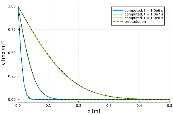

The porosity does not appear in the exact solution. On a homogeneous medium, multiplies both the accumulation and the flux, so it cancels. It no longer cancels across an interface between two materials of different porosity, which is why the model keeps it in both terms.

7. Where the Jacobian went

There is no Jacobian to write. VoronoiFVM.solve differentiates storage! and flux! with respect to u using ForwardDiff.jl, then runs its own Newton loop and adaptive time stepping. For that to work, u must be allowed to carry dual numbers instead of Float64. Do not annotate u as Float64. When a callback short-circuits, return zero(x) rather than a bare 0.0.

The models shipped with the package go one step further. Their parameter fields are type-parameterized instead of declared Float64, which lets a result be differentiated with respect to or as well as . See Parameter identification.

Summary

In the equation	In the discrete balance	Callback	Code
accumulation , built on the stored amount	, differenced in time by the solver	storage!	f[1] = m.φ * u[1]
flux		flux!	f[1] = m.D * m.φ * (u[1, 1] - u[1, 2])
at	penalty at the boundary node	bcondition!	boundary_dirichlet!(…; region = 1, value = m.c_in)
at	nothing added	—	—
one unknown	size of f and of u	nspecies, species_names	1, [:c]

Next

The examples cover one worked problem per physics. Each gives its governing equations, its material data, and the reference solution it is checked against. They use the models the package ships instead of defining their own, which is the split this page explains. Writing a model measures what that choice costs and what it buys.