Darcy column: how a pressure disturbance spreads

Connect a saturated porous column to two pressure reservoirs. Keep one end at zero reference pressure and gradually raise the pressure at the other. Water flows through the pores while pressure spreads into the interior. This example explains that transient, from conservation to the finite volume equations, and checks its final state against a simple analytical solution.

Basic derivatives, integrals, and matrix algebra are enough to follow the tutorial. Richards 1D adds changing saturation and nonlinear material laws; Biot consolidation also solves for solid displacement. Here there is only one unknown: pressure [Pa].

1. Understand the column and its loading

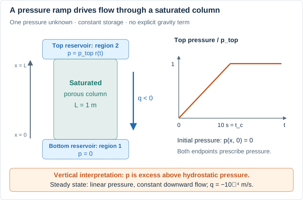
The column is drawn vertically to match the bottom/top boundary names in the code. The arrows show the pressure-driven flow direction, not computed velocities.

The coordinate runs from the bottom, , to the top, m. Both ends are open to reservoirs; the lateral surface is sealed. Cross-sectional area is constant and cancels from the one-dimensional balance.

Location	Condition	Physical meaning
Bottom, region 1		A reservoir fixes the reference pressure
Top, region 2		A second reservoir raises pressure
Whole column,		No initial pressure disturbance

Both boundary conditions are Dirichlet conditions: they prescribe pressure, not flow rate. Zero pressure at the bottom does not mean zero flow there. Saturation stays equal to one: the column already contains water before loading.

What happened to gravity?

DarcyModel implements a pressure-gradient flux with no gravity term. Taken literally, its pressure is appropriate for a horizontal column, or for a case in which gravity is deliberately neglected. For a physical vertical column with constant reference density, the same equation can instead describe excess pressure relative to hydrostatic equilibrium. With upward,

so . Under that interpretation, every pressure in this script, including the boundary data, is an excess pressure. The code does not construct the hydrostatic background. Interpreting its zero initial field as a uniform total pressure in a gravity-driven vertical column would describe a different problem.

2. Derive storage and flow from conservation

Let be the increment of stored fluid volume per bulk material volume, relative to the reference state. Linear storage means , with [Pa⁻¹] constant. For a slice of area and any interval , the volume balance in this linearized model is

Here [m/s] is the Darcy volume flux: fluid volume crossing a unit bulk area per second, positive toward increasing . It is not the pore-water velocity; for homogeneous porosity , the mean pore velocity is . Divide by and apply the balance to an arbitrarily short slice:

The mobility has units m²/(Pa·s). Intrinsic permeability has units m²; neither is the hydraulic conductivity in m/s used in a hydraulic-head formulation. Substitution gives the modeled equation:

Each term has units s⁻¹. Positive pressure gradient means negative : water moves from the high-pressure top toward the low-pressure bottom.

Storage permits a saturated material to take up additional fluid through effective compressibility. Here it is prescribed as one coefficient; the program does not calculate strain, displacement, or separate fluid and skeleton compressibilities. In Biot poroelasticity, deformation also contributes to storage. A Darcy storage coefficient used as a reduction of that model must match its mechanical constraints. This constant-storage model is also not obtained merely by setting saturation to one in this package's incompressible Richards model: that model's saturation storage becomes constant, whereas still varies with pressure here.

3. Estimate the time scale and steady state

Code field or constant	Value	Unit
`k_int`		m²
`mu_l`		Pa·s
`storativity`		Pa⁻¹
`L`	1	m
`P_TOP`		Pa

For constant coefficients the equation is , with pressure diffusivity and characteristic time

is a diffusion scale, not an exact time at which equilibrium is reached. Doubling multiplies it by four. Increasing permeability speeds the transient; increasing storage slows it. Neither changes the steady pressure profile for the same two prescribed pressures in this homogeneous column.

This example also chooses as the ramp duration: for . Thus the top reaches Pa at 10 s. The boundary value starts continuously from zero, avoiding an initial jump, but its slope changes abruptly at the end of the ramp. The ramp duration is a loading choice, not a requirement of Darcy's law.

After the ramp, steady state requires . Integrating twice and imposing both endpoint pressures gives

Steady state still has flow. Inflow at the top balances outflow at the bottom; storage no longer changes. At mid-height the steady pressure is 50,000 Pa. Once the boundary values are constant, deviations from the linear profile decay in sine modes; the slowest mode has an e-folding time s. The final time of 500 s is therefore ample for this particular case.

julia

using PoroMechanics
using VoronoiFVM
using ExtendableGrids
using Printf

4. Express the material and boundary data

DarcyModel comes from the package. Darcy's law does not change from one column to the next, so what this script owns is the geometry, the material data, and the two pressures imposed at the ends.

Both are given as data — dirichlet = ((1, 0.0), (2, ramp)). The second one is a function of time, which is how the ramp is expressed without a method of its own: PoroMechanics.dirichlet_value calls anything that is not a number with the current time. The ramp is a property of this case, not of Darcy's law.

julia

const L = 1.0          # column length [m]
const P_TOP = 1.0e5    # pressure imposed at the top [Pa]

"""Characteristic diffusion time ``t_c = S \\mu L^2 / k`` [s]."""
characteristic_time(m::DarcyModel, L) = m.storativity * m.mu_l * L^2 / m.k_int

function darcy_material(; len = L, p_top = P_TOP)
    k_int, mu_l, storativity = 1.0e-12, 1.0e-3, 1.0e-8   # [m²], [Pa·s], [Pa⁻¹]
    t_c = storativity * mu_l * len^2 / k_int
    return DarcyModel(;
        k_int, mu_l, storativity,
        dirichlet = (
            (1, 0.0),                              # bottom: p = 0
            (2, t -> p_top * min(1.0, t / t_c)),   # top: ramped to p_top over t_c
        ),
    )
end

darcy_material (generic function with 1 method)

5. From control volumes to a time step

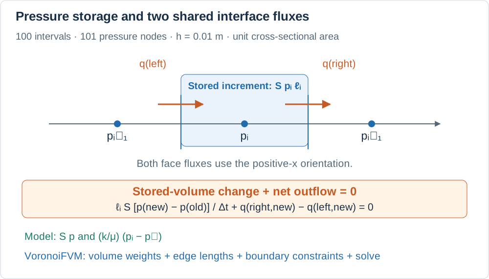
This is a schematic of an interior balance, not a computed pressure profile.

N = 100 means 100 intervals and 101 nodes, with spacing m. Each node owns a control volume extending halfway to its neighbors. Its length per unit cross-sectional area is inside and at the ends. Integrating conservation over an interior control volume gives

A shared face flux appears with opposite signs in neighboring balances. Summing the balances cancels internal exchanges, leaving storage and boundary exchange. storage! supplies and flux! supplies ; VoronoiFVM supplies volume factors, edge lengths, and global assembly. Dividing by again inside the model callback would count the geometry twice.

Backward Euler evaluates fluxes at the new time and replaces the derivative by . For an interior node on this uniform grid:

These rows form a tridiagonal linear diffusion system. Prescribed endpoint values supply the boundary constraints at the new time. VoronoiFVM uses its general implicit solver machinery even though the material laws here are linear.

The initial step and minimum step are both s; the maximum is 50 s. Δu_opt = P_TOP/10 targets a pressure change of 10,000 Pa for step adaptation. It is not an error tolerance or a strict upper bound on every accepted change. reltol controls the nonlinear solve, not the time discretization error. store_all = true retains all accepted states. The solver may take larger steps once the solution changes slowly, so saved times are generally not evenly spaced.

Backward Euler is first order in time and the centered interior flux is second order in space on this uniform grid. Stability does not guarantee that the early transient is accurately resolved.

julia

function run_darcy(; N = 100, verbose = false)
    m = darcy_material()
    t_c = characteristic_time(m, L)   # = 10 s

    # 1D grid over [0, L]
    grid = simplexgrid(range(0.0, L; length = N + 1))

    sys = fvm_system(m, grid)

    inival = unknowns(sys; inival = 0.0)

    t_end = 500.0
    dt = t_c / 20
    ctrl = VoronoiFVM.SolverControl(;
        Δt = dt,
        Δt_min = dt,
        Δt_max = t_end / 10,
        # Target pressure change for adaptive time stepping (not an error bound).
        Δu_opt = P_TOP / 10,
        store_all = true,
        reltol = 1e-6,
        verbose = verbose,
    )

    tsol = solve(sys; inival, times = (0.0, t_end), control = ctrl)

    return tsol, grid, m
end

tsol, grid, model = run_darcy()

([0.0 0.0 … 0.0 0.0;;; 5.112320893454595e-37 5.112320893454595 … 4781.278888289644 5000.0;;; 2.4051254648241346e-36 24.051254648241343 … 10652.768573774194 10999.999999999998;;; … ;;; 1.0000000000000004e-34 1000.0000000000001 … 99000.0 100000.0;;; 1.0000000000000004e-34 1000.0000000000001 … 99000.0 100000.0;;; 1.0000000000000004e-34 1000.0000000000001 … 99000.0 100000.0], ExtendableGrids.ExtendableGrid{Float64, Int32}(dim=1, nnodes=101, ncells=100, nbfaces=2), DarcyModel{Float64, Float64, Float64, Tuple{Tuple{Int64, Float64}, Tuple{Int64, Main.var"#3#4"{Float64, Float64}}}}(1.0e-12, 0.001, 1.0e-8, ((1, 0.0), (2, Main.var"#3#4"{Float64, Float64}(100000.0, 10.000000000000002)))))

6. Read the results

julia

using Plots

xcoords = grid[Coordinates][1, :]
t_c = characteristic_time(model, L)

10.000000000000002

Compare the final state with the analytical steady profile

The reported RMS is , an unweighted nodal root-mean-square error, not an integrated spatial norm. The maximum absolute error checks the worst node. Both are in Pa. The one-percent threshold below is relative to the imposed pressure amplitude, not to local pressure (which is zero at the bottom).

julia

p_ref = P_TOP .* xcoords ./ L
p_final = tsol[1, :, end]

err_L2 = sqrt(sum((p_final .- p_ref) .^ 2) / length(p_final))
err_Linf = maximum(abs.(p_final .- p_ref))

@printf("Nodes       : %d\n", length(xcoords))
@printf("t_c         : %.1f s\n", t_c)
@printf("Time steps  : %d\n", length(tsol.t) - 1)
@printf("RMS error   : %.2e Pa\n", err_L2)
@printf("L∞ error    : %.2e Pa\n", err_Linf)
err_Linf < 0.01 * P_TOP ? println("✓ err < 1 %") : println("✗ err > 1 %")

Nodes       : 101
t_c         : 10.0 s
Time steps  : 40
RMS error   : 2.61e-12 Pa
L∞ error    : 7.28e-12 Pa
✓ err < 1 %

Follow the transient profiles

The snapshots target 1, 5, 10, 20, and 50 s. For each target, we select the nearest saved state and label it with its actual time. The first two show the ramp; later curves approach the red steady profile. Pressure is on the horizontal axis and position is on the vertical axis, consistent with the geometry drawing.

julia

p = plot(;
    xlabel = "Pressure p [Pa]",
    ylabel = "Height x [m]",
    title = "Darcy 1D — pressure profiles",
    legend = :topleft,
    size = (700, 420),
)

for frac in [0.1, 0.5, 1.0, 2.0, 5.0]
    t_req = frac * t_c
    it = argmin(abs.(tsol.t .- t_req))
    plot!(p, tsol[1, :, it], xcoords; label = "t = $(round(tsol.t[it]; sigdigits = 3)) s")
end

plot!(
    p, p_ref, xcoords;
    linewidth = 3, color = :red, linestyle = :dash, label = "Analytical (t → ∞)",
)
p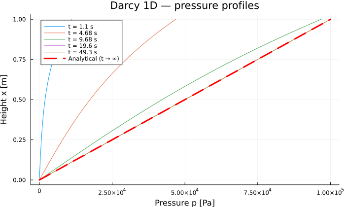

7. Checks, limitations, and short exercises

A small final error checks the boundary data, flux sign, and long-time behavior. It does not establish transient convergence: a linear steady profile is represented exactly by this spatial stencil, and early time errors have decayed by 500 s. For a transient convergence study, compare common physical times while refining the grid and reducing the time-step limits separately.

From the repository root, with Julia 1.12 or newer and the examples environment prepared, run julia --project=examples examples/darcy_column/run.jl. In a Julia session started with julia --project=examples:

julia

include("examples/darcy_column/run.jl")  # also runs the default case
tsol_fine, grid_fine, model_fine = run_darcy(N = 200)

run_darcy exposes grid resolution and verbosity. To vary time resolution, edit its SolverControl settings; changing N alone does not refine time. If material coefficients are changed in darcy_material, remember that the ramp duration also changes with . Hold the loading schedule fixed when the aim is to isolate the influence of a material parameter under the same experiment.

Flux sign: use the steady profile to recover m/s. For an area of 0.01 m², the discharge magnitude is m³/s. Explain why a zero bottom pressure permits this outflow.
Storage: a uniform 10,000 Pa pressure increase would give . This is additional stored fluid volume per bulk volume, not a saturation increase above one.
Time scale: halve permeability. The diffusion scale and, in this script, the ramp duration both double; the final pressure is unchanged and the steady discharge magnitude halves.
Conservation: sum the interior finite volume balances and identify the two remaining boundary exchanges. Include endpoint storage when writing a balance for the whole column. Reservoir fluxes at prescribed-pressure nodes are not zero-flux conditions.
Model choice: a layered column with different permeabilities has continuous steady flux and piecewise linear pressure. The single straight-line reference used here no longer applies. Unsaturated flow or a displacement prediction also requires a different model.

The regression suite checks reproducibility against a stored solution; it is separate from a mesh or time convergence study. Run it with julia --project -e 'using Pkg; Pkg.test(test_args=["regression"])'. Regenerate the conceptual drawings with python3 examples/darcy_column/draw_schematics.py.

Darcy column: how a pressure disturbance spreads ​

1. Understand the column and its loading ​

What happened to gravity? ​

2. Derive storage and flow from conservation ​

3. Estimate the time scale and steady state ​

4. Express the material and boundary data ​

5. From control volumes to a time step ​

6. Read the results ​

Compare the final state with the analytical steady profile ​

Follow the transient profiles ​

7. Checks, limitations, and short exercises ​

Darcy column: how a pressure disturbance spreads

1. Understand the column and its loading

What happened to gravity?

2. Derive storage and flow from conservation

3. Estimate the time scale and steady state

4. Express the material and boundary data

5. From control volumes to a time step

6. Read the results

Compare the final state with the analytical steady profile

Follow the transient profiles

7. Checks, limitations, and short exercises