Mandel's Problem

The benchmark that separates a genuinely coupled poroelastic solver from one that merely solves two equations side by side. A rectangular sample is squeezed between two rigid, frictionless, impermeable plates and drained through its lateral faces. The pore pressure at the centre does not decay: it rises above its initial value before falling — the Mandel–Cryer effect (Mandel, 1953).

The overshoot is produced by the rigidity of the plates. As the edges drain, the material there stiffens (drained response) while the centre is still undrained and soft, so the plate transfers load towards the centre and raises the pressure there. A solver that gets the coupling term wrong reproduces a monotone decay and looks plausible — which is exactly why this case is worth the trouble.

Problem

A sample   ,    in plane strain. At   a constant vertical force is applied through rigid plates at   ; the faces    are drained and traction-free. Only a quarter is meshed,  ,  , with symmetry conditions on the two inner edges.

Boundary	Condition
	symmetry:  , no flow
	symmetry:  , no flow
	drained  , traction free
	rigid plate: uniform but unknown, carrying the total force

The rigid plate is the whole difficulty. Its displacement is not prescribed and not free either: every node on the top edge must share one unknown. That is imposed here with Ferrite affine constraints tying each top to a single master dof, on which the resultant force is applied.

Reference solution

With the positive roots of

the pore pressure is (Cheng and Detournay, 1988)

and the initial value is uniform,   .

Because    , the first root lies in and the remaining ones in  . That first root is the dominant term; omitting it — an easy mistake, since the later roots follow a tidier pattern — turns the solution negative and destroys the overshoot.

include("biot_common.jl")

uniform_schedule (generic function with 1 method)

Model

Parameters chosen for a pronounced effect:   and   against a drained  . The overshoot grows with  , and vanishes when the two coincide.

const MANDEL_MATERIAL = HomogeneousBiot(;
    E = 1.0e8, nu = 0.2, k = 1.0e-13, mu_l = 1.0e-3, b = 1.0, N = 7.2e-9,
)

const A_HALF = 1.0    # sample half-width [m]
const B_HALF = 1.0    # sample half-height [m]
const F_TOTAL = 1.0e6 # vertical force carried by the quarter [N/m]

"""Initial uniform pore pressure ``p_0 = F B (1+\\nu_u)/(3a)`` [Pa]."""
initial_pressure(m::HomogeneousBiot, F = F_TOTAL, a = A_HALF) =
    F * skempton(m) * (1 + undrained_poisson(m)) / (3a)

initial_pressure (generic function with 3 methods)

Reference series

"""
    mandel_roots(m; nterms = 60)

Positive roots of ``\\tan\\alpha = \\frac{1-\\nu}{\\nu_u-\\nu}\\alpha``, one per interval
``((n-1)\\pi,\\ (n-1)\\pi + \\pi/2)``, by bisection.
"""
function mandel_roots(m::HomogeneousBiot; nterms = 60)
    k = (1 - m.nu) / (undrained_poisson(m) - m.nu)
    f(α) = tan(α) - k * α
    roots = Float64[]
    for n in 1:nterms
        lo = (n - 1) * π + 1.0e-12
        hi = (n - 1) * π + π / 2 - 1.0e-12
        flo = f(lo)
        f(lo) * f(hi) > 0 && continue
        for _ in 1:200
            mid = (lo + hi) / 2
            if f(mid) * flo <= 0
                hi = mid
            else
                lo = mid
                flo = f(mid)
            end
        end
        push!(roots, (lo + hi) / 2)
    end
    return roots
end

"""
    mandel_pressure(m, roots, x, T; F, a) -> p [Pa]

Pore pressure at position `x` and dimensionless time `T = c t / a²`.
"""
function mandel_pressure(m::HomogeneousBiot, roots, x, T; F = F_TOTAL, a = A_HALF)
    pref = 2 * F * skempton(m) * (1 + undrained_poisson(m)) / (3a)
    s = 0.0
    for α in roots
        s += (sin(α) / (α - sin(α) * cos(α))) *
            (cos(α * x / a) - cos(α)) * exp(-α^2 * T)
    end
    return pref * s
end

mandel_pressure (generic function with 1 method)

Solving

"""
    run_mandel(; m, nelx, nely, T_probe, T_start, dT)

Returns `(m, xs, T_probe, profiles, T_hist, p_centre)`. `profiles[i]` is the pressure at the
nodes `xs` at time `T_probe[i]`; `p_centre` is the pressure at `x = 0` at every step, which
is what exhibits the overshoot.
"""
function run_mandel(;
        m = MANDEL_MATERIAL,
        nelx = 60,
        nely = 4,
        T_probe = [0.01, 0.05, 0.1, 0.3, 0.6, 1.0],
        T_start = 1.0e-4,
        dT = 5.0e-4,
    )
    c = consolidation_coefficient(m)
    t_of_T(T) = T * A_HALF^2 / c

    grid = generate_grid(Quadrilateral, (nelx, nely), Vec(0.0, 0.0), Vec(A_HALF, B_HALF))

    ip_geo = Lagrange{RefQuadrilateral, 1}()
    ip_u = Lagrange{RefQuadrilateral, 1}()^2
    ip_p = Lagrange{RefQuadrilateral, 1}()

    dh = DofHandler(grid)
    add!(dh, :u, ip_u)
    add!(dh, :p, ip_p)
    close!(dh)

    qr = QuadratureRule{RefQuadrilateral}(2)
    cv_u = CellValues(qr, ip_u, ip_geo)
    cv_p = CellValues(qr, ip_p, ip_geo)

    maps = node_dof_maps(dh, grid, (:u, 2), :p)
    uy_dof, p_dof = maps.u, maps.p

    coords = [node.x for node in grid.nodes]
    tol = 1.0e-9
    top_nodes = findall(cc -> abs(cc[2] - B_HALF) < tol, coords)
    master_node = top_nodes[argmin(coords[n][1] for n in top_nodes)]
    master_dof = uy_dof[master_node]

    # Symmetry, drainage, and the rigid plate
    ch = ConstraintHandler(dh)
    add!(ch, Dirichlet(:u, getfacetset(grid, "left"), (x, t) -> 0.0, [1]))
    add!(ch, Dirichlet(:u, getfacetset(grid, "bottom"), (x, t) -> 0.0, [2]))
    add!(ch, Dirichlet(:p, getfacetset(grid, "right"), (x, t) -> 0.0))
    for n in top_nodes
        n == master_node && continue
        add!(ch, AffineConstraint(uy_dof[n], [master_dof => 1.0], 0.0))
    end
    close!(ch)
    update!(ch, 0.0)

    n_loc = ndofs_per_cell(dh)
    # The sparsity pattern must accommodate the affine coupling between master and slaves.
    K1 = allocate_matrix(dh, ch)
    K2 = allocate_matrix(dh, ch)
    A = allocate_matrix(dh, ch)
    as1 = start_assemble(K1)
    as2 = start_assemble(K2)
    ke1 = zeros(n_loc, n_loc)
    ke2 = zeros(n_loc, n_loc)

    for cell in CellIterator(dh)
        reinit!(cv_u, cell)
        reinit!(cv_p, cell)
        biot_element_matrices!(ke1, ke2, m, cv_u, cv_p)
        assemble!(as1, celldofs(cell), ke1)
        assemble!(as2, celldofs(cell), ke2)
    end

    # The whole resultant is applied to the master dof: every top node shares its
    # displacement, so the virtual work of the load is F · δu_master.
    f_ext = zeros(ndofs(dh))
    f_ext[master_dof] = -F_TOTAL

    xs = [cc[1] for cc in coords]
    centre_nodes = findall(cc -> abs(cc[1]) < tol, coords)

    schedule = uniform_schedule(T_probe; T_start = T_start, dT = dT)

    x = zeros(ndofs(dh))
    apply!(x, ch)

    profiles = Vector{Vector{Float64}}()
    probes_left = sort(T_probe)
    T_hist = Float64[]
    p_centre = Float64[]
    t_prev = 0.0

    for T in schedule
        t = t_of_T(T)
        dt = t - t_prev
        combine!(A, K1, K2, 1.0 / dt)
        rhs = copy(f_ext)
        mul!(rhs, K2, x, 1.0 / dt, 1.0)
        apply!(A, rhs, ch)
        x = A \ rhs
        apply!(x, ch)      # fill the tied dofs back in
        t_prev = t

        push!(T_hist, T)
        push!(p_centre, sum(x[p_dof[n]] for n in centre_nodes) / length(centre_nodes))

        if !isempty(probes_left) && isapprox(T, probes_left[1]; rtol = 1.0e-9)
            push!(profiles, [x[p_dof[i]] for i in 1:getnnodes(grid)])
            popfirst!(probes_left)
        end
    end

    return m, xs, sort(T_probe), profiles, T_hist, p_centre
end

model, xs, T_probe, p_num, T_hist, p_centre = run_mandel()

(BiotPoroelastic{Float64}(1.0e8, 0.2, 1.0e-13, 0.001, 1.0, 7.2e-9), [0.0, 0.016666666666666663, 0.033333333333333326, 0.04999999999999999, 0.06666666666666665, 0.08333333333333331, 0.09999999999999998, 0.1166666666666667, 0.1333333333333333, 0.15000000000000002  …  0.85, 0.8666666666666667, 0.8833333333333333, 0.9, 0.9166666666666666, 0.9333333333333333, 0.95, 0.9666666666666667, 0.9833333333333333, 1.0], [0.01, 0.05, 0.1, 0.3, 0.6, 1.0], [[342893.94983298786, 342893.9497657222, 342893.94954644865, 342893.9491184845, 342893.9483722257, 342893.9471189109, 342893.945046092, 342893.94164517557, 342893.936095689, 342893.92708231625  …  246676.1746365053, 227469.40252878133, 205862.70582622258, 181890.8835058291, 155665.47283479368, 127377.97380454048, 97298.22163190611, 65767.53867513326, 33186.79106100615, 0.0], [354273.01922553364, 354256.62591183034, 354207.1366951883, 354123.62178735837, 354004.52505161025, 353847.65444045776, 353650.1689528976, 353408.5624555728, 353118.6448103754, 352775.5208484655  …  132736.64136537345, 119074.10235342928, 105064.75437853763, 90737.91787744618, 76125.13453178189, 61259.934292035345, 46177.57585473875, 30914.763920896043, 15509.347012259152, 0.0], [347589.2279008634, 347518.252351428, 347305.1164911493, 346949.19398396375, 346449.44526647596, 345804.42403313005, 345012.2862954113, 344070.80199449067, 342977.36914005684, 341729.0304408598  …  99498.1031991415, 88931.0287056862, 78213.18751408323, 67356.30570170537, 56372.540944577595, 45274.434897987616, 34074.86300235014, 22786.982063934705, 11424.175980606004, 0.0], [247342.50758247293, 247262.1141204019, 247020.9734184171, 246619.204529877, 246057.00587916098, 245334.65526437483, 244452.50986021184, 243411.0062200459, 242210.66027608328, 240852.06733615324  …  60385.41848895243, 53875.515020224644, 47307.16459129196, 40683.98471609155, 34009.62659157301, 27287.77264662846, 20522.13405222575, 13716.448197187694, 6874.476134102464, 0.0], [138325.01748056806, 138279.72813675803, 138143.88451923535, 137917.55985659335, 137600.87615272767, 137194.00412122108, 136697.16309353142, 136110.62090102764, 135434.69373093988, 134669.74595629427  …  33660.712403238846, 30030.752094632015, 26368.601156253364, 22676.23429614897, 18955.64252076891, 15208.832060702365, 11437.823288165735, 7644.649626835384, 3831.3564546270945, 0.0], [63654.100941767196, 63633.259375014546, 63570.74591230026, 63466.594260197184, 63320.86057613211, 63133.6234381068, 62904.98380233026, 62635.064948783205, 62324.01241474669, 61971.99391633231  …  15489.77389727296, 13819.360262205142, 12134.133840296781, 10435.00328722703, 8722.884755630312, 6998.701401118361, 5263.382884525211, 3517.864870644972, 1763.088523722389, 0.0]], [0.0001, 0.0006000000000000001, 0.0011, 0.0016, 0.0021, 0.0026, 0.0031, 0.0036, 0.0041, 0.0046  …  0.9956, 0.9961, 0.9966, 0.9971, 0.9976, 0.9981, 0.9986, 0.9991, 0.9996, 1.0], [334210.78809155634, 335480.41267740907, 336328.9573532658, 337000.40530295833, 337572.1066708312, 338078.34583831194, 338537.56103648554, 338960.94587224245, 339355.877877107, 339727.5158663231  …  64199.885066125564, 64137.62976274729, 64075.43482898454, 64013.30020629476, 63951.22583619667, 63889.2116602602, 63827.257620117256, 63765.36365745014, 63703.529714003336, 63654.10094174923])

Results

using Plots

roots = mandel_roots(model)
p0 = initial_pressure(model)

@printf("Skempton B        : %.6f\n", skempton(model))
@printf("Undrained ν_u     : %.6f   (drained ν = %.3f)\n", undrained_poisson(model), model.nu)
@printf("Diffusivity c     : %.6e m²/s\n", consolidation_coefficient(model))
@printf("Initial pressure p₀: %.6e Pa\n", p0)
@printf("First five roots  : %s\n", join(round.(roots[1:5]; digits = 5), ", "))
println()

Skempton B        : 0.714286
Undrained ν_u     : 0.400000   (drained ν = 0.200)
Diffusivity c     : 6.172840e-03 m²/s
Initial pressure p₀: 3.333333e+05 Pa
First five roots  : 1.39325, 4.65878, 7.82203, 10.97279, 14.11946

The Mandel–Cryer overshoot

The quantity that matters. A monotone curve here would mean the coupling is wrong.

p_centre_ref = [mandel_pressure(model, roots, 0.0, T) for T in T_hist]

i_peak = argmax(p_centre)
i_peak_ref = argmax(p_centre_ref)
@printf("numerical peak : p/p₀ = %.5f at T = %.4f\n", p_centre[i_peak] / p0, T_hist[i_peak])
@printf("reference peak : p/p₀ = %.5f at T = %.4f\n", p_centre_ref[i_peak_ref] / p0, T_hist[i_peak_ref])
@printf("overshoot      : %.2f %% above p₀\n", 100 * (p_centre_ref[i_peak_ref] / p0 - 1))
println()

plt_hist = plot(
    T_hist, p_centre_ref ./ p0;
    xlabel = "T = c t / a²  [-]", ylabel = "p(0, t) / p₀  [-]",
    title = "Mandel–Cryer effect at the centre",
    label = "reference series", lw = 2, color = :black,
    xscale = :log10, legend = :bottomleft, size = (700, 420),
)
plot!(
    plt_hist, T_hist[1:8:end], (p_centre ./ p0)[1:8:end];
    seriestype = :scatter, ms = 3, mswidth = 0, color = :crimson, label = "finite elements",
)
hline!(plt_hist, [1.0]; ls = :dash, color = :grey, label = "p₀")
plt_hist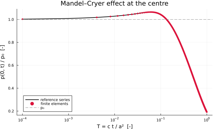

Error against the reference

println("      T     |  L2 error  |  L∞ error [Pa]")
println("-"^44)
errors = Float64[]
for (T, pn) in zip(T_probe, p_num)
    ref = [mandel_pressure(model, roots, x, T) for x in xs]
    e2 = norm(pn .- ref) / norm(ref)
    push!(errors, e2)
    @printf("  %8.4f  |  %.3e |  %10.2f\n", T, e2, maximum(abs.(pn .- ref)))
end
println("-"^44)
@printf("worst relative L2 error: %.3e\n", maximum(errors))

      T     |  L2 error  |  L∞ error [Pa]
--------------------------------------------
    0.0100  |  2.404e-03 |     2162.02
    0.0500  |  7.946e-04 |      427.84
    0.1000  |  4.918e-04 |      205.38
    0.3000  |  3.131e-04 |       70.80
    0.6000  |  5.484e-04 |       75.85
    1.0000  |  8.609e-04 |       54.78
--------------------------------------------
worst relative L2 error: 2.404e-03

Pressure profiles

plt = plot(;
    xlabel = "x / a  [-]", ylabel = "p / p₀  [-]",
    title = "Mandel — pressure profiles",
    legend = :bottomleft, size = (700, 440),
)

xfine = range(0, A_HALF; length = 300)
order = sortperm(xs)
palette = cgrad(:viridis, max(length(T_probe), 2); categorical = true)

for (i, (T, pn)) in enumerate(zip(T_probe, p_num))
    plot!(
        plt, xfine ./ A_HALF, [mandel_pressure(model, roots, x, T) / p0 for x in xfine];
        color = palette[i], lw = 2, label = "T = $T",
    )
    plot!(
        plt, (xs ./ A_HALF)[order], (pn ./ p0)[order];
        color = palette[i], seriestype = :scatter, ms = 2, mswidth = 0, label = "",
    )
end
plt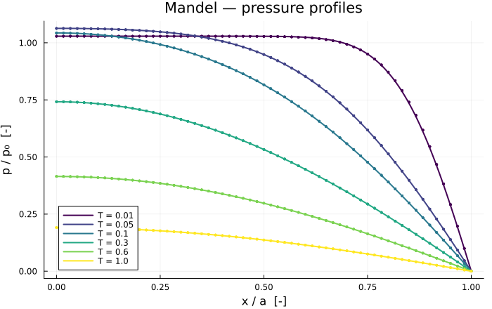

Notes

• The rigid plate is the physics — replace the affine constraints by a uniform traction and the overshoot disappears entirely. The plate is what transfers load from the drained edges to the undrained core.

• The first root — with     there is a root in , outside the   pattern of all the others. It is the slowest-decaying and therefore dominant term.

• Series truncation at   — the expansion converges slowly at very small time; at   the 60-term sum returns   rather than . The probe times start at  , where truncation is far below the discretisation error.

• Sparsity with affine constraints — the matrix has to be allocated with allocate_matrix(dh, ch), not allocate_matrix(dh), or the master–slave couplings have nowhere to go.