Identifying a diffusion coefficient

The Fickian diffusion example solves the forward problem: given the diffusion coefficient and the concentration imposed at the inlet, compute the concentration profile. A laboratory faces the opposite question. It measures a few concentrations at a few depths, for instance on slices ground from a core, and wants the and that explain them. This is the inverse problem.

It is solved here by least squares: find the parameters that minimize

Gauss–Newton and Levenberg–Marquardt iterations need the Jacobian  , which tells how each simulated measurement moves when a parameter moves. Every simulated value comes out of a full transient finite volume solve, so this Jacobian is the derivative of the solve. It is computed by automatic differentiation, with ForwardDiff, which the next section explains.

The page answers four questions in turn:

1. how the physical experiment becomes a discrete forward model;

2. how to differentiate that model and check its sensitivities;

3. which parameters the measurements can determine;

4. how to calibrate them and assess uncertainty and numerical bias.

Basic derivatives and matrix algebra are enough to follow the derivations below. The dual-number examples introduce automatic differentiation from first principles. Run the whole script from the repository root with Julia 1.12 or newer: julia --project=examples examples/fickian_identification/run.jl, after preparing the examples environment. It prints sensitivity, calibration, and refinement tables and creates a plot of the fitted profiles.

using PoroMechanics
using VoronoiFVM
using ExtendableGrids
using OrdinaryDiffEq
using ForwardDiff
using SpecialFunctions
using LinearAlgebra
using Random
using Printf
using Plots

1. Define the experiment and the forward equation

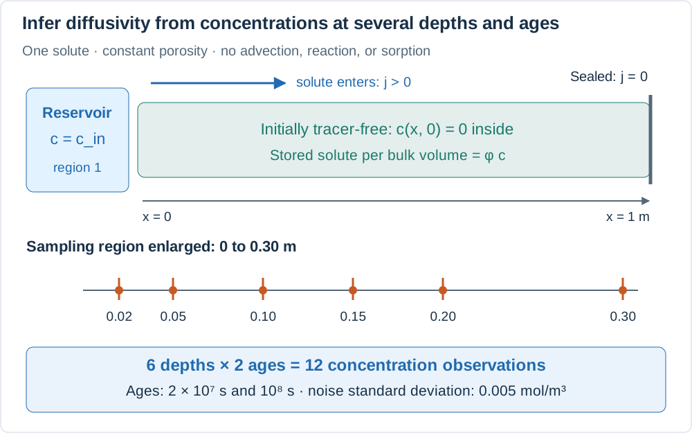
Sampling locations are shown along a homogeneous specimen. The drawing describes the experiment; it is not a simulated concentration profile.

A saturated, homogeneous specimen is initially free of tracer. Its left face contacts a reservoir with constant concentration . The right face is sealed. Water does not advect: solute moves only by diffusion, with no reaction, sorption, or change of porosity. The unknown [mol/m³] is solute concentration per unit pore-solution volume. Stored solute per bulk volume is . This distinction matters when deciding whether porosity is identifiable.

Location or quantity	Condition or value	Meaning
, region 1	for	Prescribed inlet concentration
, region 2		Sealed end; no solute crosses it
Interior,		No initial tracer
	1 m	Finite specimen length
	0.30	Fixed, uniform pore-volume fraction
Reference	m²/s	Diffusivity used to generate synthetic data
Reference	1 mol/m³	Reservoir value used to generate data

Define solute flux [mol/(m²·s)] per unit bulk cross-sectional area, positive toward increasing . For any slice of constant area , conservation and Fick's law give

Dividing by area and shrinking the slice yields

For constant and , this reduces to  . In this package's convention, the coefficient multiplying the concentration gradient in the bulk-area flux is ; a reported experimental diffusion coefficient must use the same convention before being compared with . The initially decreasing concentration gives  : tracer enters from the left.

From a continuous profile to twelve predicted measurements

On a uniform grid with intervals, spacing  , and control-volume length , integrate the balance around node :

Inside the grid  , giving    ; endpoint volumes have length . The inlet value is imposed, while the sealed endpoint has zero external flux. The FickModel storage callback supplies and its flux callback supplies  . VoronoiFVM supplies geometric factors and assembles the spatial system. OrdinaryDiffEq advances that system in time below.

A measurement operator then samples the computed profile. Six depths at two ages give a vector of 12 predictions, ordered first by age and then by depth. Here simulate selects the nearest node to each requested depth. All six depths coincide with nodes on the 100-, 200-, and 400-interval grids used on this page, so this selection introduces no location error in the reported refinement study. For arbitrary depths, interpolate explicitly. For concentrations averaged over ground slices, average the simulation over the same slices: a point value and a slice average are different observables.

2. Understand automatic differentiation

There are three ways to get the derivative of a computed result with respect to a parameter.

• Finite differences run the computation twice, at and at  , and divide the change by . The result is an approximation, and its error depends on : too large and the slope is wrong, too small and rounding errors dominate.

• Symbolic differentiation writes out the formula of the derivative. That is impractical for a result that comes out of a mesh, a Newton loop and a thousand time steps.

• Automatic differentiation applies the rules of differentiation to every elementary operation the computation performs, as it performs them. The result is the exact derivative along the executed differentiable operations, up to rounding, with no finite-difference step to choose. Mesh and time-integration errors still remain.

ForwardDiff implements the forward mode with dual numbers. A dual number carries a value and a derivative, written   with the rule  . Arithmetic on dual numbers applies the differentiation rules by itself:

The first is the product rule, the second the chain rule.

Take   at  . The computation starts from its input, so the input must already carry a derivative for the rules to propagate. That derivative is the seed: the derivative of the input with respect to the variable chosen for differentiation. To differentiate with respect to itself, the seed is  .

a = ForwardDiff.Dual(2.0, 1.0)     # x = 2, seeded with dx/dx = 1: differentiate with respect to x
fa = a^2 * exp(a)

Dual{Nothing}(29.5562243957226,59.1124487914452)

Each operation passes the derivative along:

quantity	value	derivative part
		(the seed)

The computation never used a formula for . It only applied the product rule and the chain rule to each operation, with numbers, as the last column shows. The formula     appears here only to check the result: at   it gives  , the derivative part found above. For the finite volume solve below, no such formula exists to check against, and the derivative is compared with finite differences instead.

Without the seed of 1, the chain would have no derivative to multiply.

The seed says with respect to what the derivative is taken:

seed	meaning	derivative part
1	is the variable,
0	is a constant
3	, derivative with respect to

for seed in (1.0, 0.0, 3.0)
    z = ForwardDiff.Dual(2.0, seed)
    @printf("seed %.0f  ->  derivative part %.2f\n", seed, ForwardDiff.partials(z^2 * exp(z))[1])
end

seed 1  ->  derivative part 59.11
seed 0  ->  derivative part 0.00
seed 3  ->  derivative part 177.34

With several parameters, each one gets its own seed. For , the first carries the derivative parts and the second . Each result then carries two derivative parts, which form its row of the Jacobian. ForwardDiff.derivative and ForwardDiff.jacobian set these seeds and read the results for you. Writing Dual by hand, as above, only serves to show the mechanism:

ForwardDiff.derivative(x -> x^2 * exp(x), 2.0)

59.1124487914452

Nothing changes for a longer computation. Every addition, product, exp, linear solve and time step in the finite volume code passes the part along. At the end, the part of each simulated concentration is its derivative with respect to the seeded parameter. With several parameters, a dual number carries one part per parameter, and all of them travel through a single run. That is what ForwardDiff.jacobian does.

Two levels of automatic differentiation are nested in this page, and they do not interfere:

1. VoronoiFVM differentiates storage! and flux! with respect to the unknowns, to build the Jacobian of its Newton iterations.

2. This page differentiates the whole solve with respect to the parameters and , to build the Jacobian of the least-squares problem.

ForwardDiff labels each level with its own tag, so the two kinds of are never mixed up.

Automatic differentiation also has a reverse mode, provided by other packages such as Zygote or Enzyme.

	forward mode (ForwardDiff)	reverse mode
cost	about one computation per parameter, carried together	about one computation per output
suited to	few parameters	many parameters and one scalar output, such as a cost function
memory	state plus propagated partial derivatives	intermediates stored or recomputed

With two parameters, the forward mode is the right choice. The reverse mode would pay off if, say, were identified cell by cell, with hundreds of parameters for a single cost .

Adaptive step selection and stopping tests can change the executed path. Therefore, differentiating a numerical solve does not by itself certify the sensitivity of the continuous PDE. We check derivatives numerically and later refine the spatial model; time tolerances also need checking if greater precision is required. All intermediate arrays must accept the parameter's numeric type. Explicitly converting a dual number to Float64 would break this propagation; see the ForwardDiff limitations.

3. Generate and interpret the measurements

Six depths are sampled at two ages, about eight months and about three years.

The measurements are synthetic. They come from the analytical solution

with   m²/s and   mol/m³, and not from the finite volume model that is fitted to them. Data generated by the fitted model itself would be reproduced exactly, which would hide the discretization error. Analytical data keep that error visible, and it matters in the last section.

This complementary-error-function solution is exact on a semi-infinite domain   with zero initial concentration and a constant inlet. The fitted model uses a finite domain with a sealed end. They agree to high accuracy at the sampled depths only while the far boundary has negligible influence. At the latest age,   m and  ; the semi-infinite concentration at 1 m is only    mol/m³. This supports using the analytical profile here, but it is not a general identity between the two boundary-value problems. A shorter specimen, later age, or much larger diffusivity would require revisiting the reference solution.

Independent Gaussian measurement noise with standard deviation 0.005 mol/m³, half a percent of , is added using a fixed random seed. The two ages are   s (about 231 days) and s (about 1,157 days). At the deepest, earliest point the expected concentration is smaller than the noise, so a noisy observation can be negative. That is possible under this additive measurement model even though the underlying concentration is nonnegative.

const D_TRUE = 1.0e-10    # diffusion coefficient used to generate the data [m²/s]
const C_IN_TRUE = 1.0     # inlet concentration used to generate the data [mol/m³]
const PHI = 0.30          # porosity [-]
const L = 1.0             # length of the column [m]
const SIGMA = 0.005       # standard deviation of the measurement noise [mol/m³]

const X_OBS = [0.02, 0.05, 0.10, 0.15, 0.20, 0.30]    # measurement depths [m]
const T_OBS = [2.0e7, 1.0e8]                          # measurement ages [s]

analytical(D, c_in, x, t) = c_in * erfc(x / (2 * sqrt(D * t)))

# Measurements are ordered by age, then by depth, and every function below uses that order.
Random.seed!(2026)
c_exact = [analytical(D_TRUE, C_IN_TRUE, x, t) for t in T_OBS for x in X_OBS]
c_obs = c_exact .+ SIGMA .* randn(length(c_exact))

4. Build a differentiable transient solve

To differentiate with respect to and , those two numbers are replaced by dual numbers. Everything computed from them must then be able to hold dual numbers as well:

• the model: FickModel takes the type of its coefficients as a parameter, so a dual is accepted as is;

• the unknowns: fvm_system(...; valuetype = T) builds a system whose values have type T.

In the dependency setup documented here, the usual VoronoiFVM call solve(sys; inival, times, control) does not support this parameter-dual path. VoronoiFVM chooses each time step from the change of the previous one (see Getting Started). That change is a dual number, so the next step and then the time itself become dual numbers too. VoronoiFVM stores the time in a Float64 field, and the solve stops with MethodError(Float64, Dual(…)). Fixed time steps do not avoid it. Differentiating a solve records the details.

The way around it keeps VoronoiFVM for the space discretization and hands the time stepping to OrdinaryDiffEq. ODEProblem(sys, inival, tspan) turns the finite volume system into a system of ordinary differential equations. VoronoiFVM still evaluates storage!, flux! and bcondition!, and still differentiates them for the Jacobian. OrdinaryDiffEq integrates in time, and its step-size control is written to carry dual numbers.

Rosenbrock23 is a linearly implicit method, stable on stiff problems such as diffusion. saveat = T_OBS keeps only the solution at the measurement ages, and reshape(sol, sys) turns the result into the familiar tsol[species, node, step] form.

"""
    solve_profiles(D, c_in; phi = PHI, N = 100) -> (x, tsol)

Concentration profiles at the ages `T_OBS`, on a grid of `N` cells. `D`, `c_in` and `phi`
may be dual numbers.
"""
function solve_profiles(D, c_in; phi = PHI, N = 100)
    T = promote_type(typeof(D), typeof(c_in), typeof(phi))
    grid = simplexgrid(range(0, L; length = N + 1))

    model = FickModel(; phi, D, dirichlet = ((1, c_in),))
    sys = fvm_system(model, grid; valuetype = T)

    inival = unknowns(sys; inival = zero(T))
    inival[1, 1] = c_in    # consistent with the Dirichlet value, as in the forward example

    problem = ODEProblem(sys, inival, (0.0, T_OBS[end]))
    sol = OrdinaryDiffEq.solve(
        problem, Rosenbrock23();
        abstol = 1.0e-9, reltol = 1.0e-7, saveat = T_OBS,
    )
    return grid[Coordinates][1, :], reshape(sol, sys)
end

"Simulated concentrations at the measurement points, in the order of `c_obs`."
function simulate(D, c_in; phi = PHI, N = 100)
    x, tsol = solve_profiles(D, c_in; phi, N)
    nodes = [argmin(abs.(x .- xo)) for xo in X_OBS]
    steps = [findfirst(==(t), tsol.t) for t in T_OBS]
    return [tsol[1, k, n] for n in steps for k in nodes]
end

The parameters are dimensionless and scaled to be of order one:   and  , where   m²/s and   mol/m³. The code uses concentrations numerically in mol/m³, so multiplying the second component by the numerical scale 1 is implicit. Without scaling, the two sensitivity columns carry very different numerical scales because of the units. A raw condition number would then be dominated by that choice. Scaling gives interpretable parameter directions and step sizes; the diagonal damping used below provides additional curvature scaling.

simulate(θ::AbstractVector; kwargs...) = simulate(θ[1] * 1.0e-10, θ[2]; kwargs...)
θ_true = [D_TRUE / 1.0e-10, C_IN_TRUE]

5. Check the derivatives

The Jacobian from ForwardDiff is compared with central differences,    . Differences cost two extra solves per parameter and depend on the step . ForwardDiff needs one solve carrying two partial derivatives, and has no step to choose.

J_ad = ForwardDiff.jacobian(simulate, θ_true)
J_fd = reduce(
    hcat, map(1:2) do k
        h = 1.0e-6
        e = [i == k ? h : 0.0 for i in 1:2]
        (simulate(θ_true .+ e) .- simulate(θ_true .- e)) ./ (2h)
    end
)

println("  t [s]   x [m]   ∂c/∂θ₁ ForwardDiff   ∂c/∂θ₁ differences   ∂c/∂θ₂ ForwardDiff   ∂c/∂θ₂ differences")
for (i, (t, x)) in enumerate((t, x) for t in T_OBS for x in X_OBS)
    @printf(
        "  %.0e  %.2f   %+.8e      %+.8e      %+.8e      %+.8e\n",
        t, x, J_ad[i, 1], J_fd[i, 1], J_ad[i, 2], J_fd[i, 2]
    )
end

  t [s]   x [m]   ∂c/∂θ₁ ForwardDiff   ∂c/∂θ₁ differences   ∂c/∂θ₂ ForwardDiff   ∂c/∂θ₂ differences
  2e+07  0.02   +1.20308120e-01      +1.20309018e-01      +7.51603660e-01      +7.51604067e-01
  2e+07  0.05   +2.30650224e-01      +2.30651365e-01      +4.29017724e-01      +4.29018232e-01
  2e+07  0.10   +1.79640911e-01      +1.79640574e-01      +1.14415029e-01      +1.14414867e-01
  2e+07  0.15   +5.68837283e-02      +5.68834167e-02      +1.82497477e-02      +1.82496176e-02
  2e+07  0.20   +8.87554482e-03      +8.87560366e-03      +1.72409787e-03      +1.72412586e-03
  2e+07  0.30   +3.47753798e-05      +3.47808647e-05      +3.33026512e-06      +3.33236549e-06
  1e+08  0.02   +5.58910935e-02      +5.58913272e-02      +8.87514440e-01      +8.87514576e-01
  1e+08  0.05   +1.32564269e-01      +1.32564788e-01      +7.23625686e-01      +7.23625986e-01
  1e+08  0.10   +2.19706954e-01      +2.19707610e-01      +4.79454936e-01      +4.79455306e-01
  1e+08  0.15   +2.40974312e-01      +2.40974690e-01      +2.88857416e-01      +2.88857614e-01
  1e+08  0.20   +2.07337829e-01      +2.07337801e-01      +1.57385861e-01      +1.57385826e-01
  1e+08  0.30   +8.91283101e-02      +8.91280450e-02      +3.40246314e-02      +3.40244893e-02

Read the columns together: agreement should be assessed in both absolute and relative terms. At 0.30 m at the first age, the analytical concentration is only about   mol/m³, so relative derivative errors can be large even when absolute errors are small. Finite-difference accuracy depends on both and solver tolerances. Repeat with several values to seek an agreement plateau; ever smaller differences eventually amplify numerical error.

The second column also has an exact answer. The problem is linear in : doubling the inlet concentration doubles the whole profile, so  , which at   is the simulated concentration itself.

c_sim = simulate(θ_true)
@printf("max |∂c/∂c_in − c / c_in| = %.1e\n", maximum(abs.(J_ad[:, 2] .- c_sim)))

max |∂c/∂c_in − c / c_in| = 3.1e-08

The printed gap is an absolute sensitivity discrepancy. It is affected by time integration and adaptive control; it is not itself the solver relative tolerance. Tightening tolerances should be checked before interpreting very small differences.

6. Ask which parameters the measurements can determine

A parameter is determined by the data only if changing it changes the simulated measurements. Locally, this is read from the Jacobian: a zero column or a linear combination of other columns signals a parameter direction that these measurements cannot distinguish to first order. Its singular values quantify this sensitivity. A singular value close to zero means a direction in scaled parameter space along which predictions barely move to first order. Full column rank establishes local sensitivity, not global uniqueness.

The porosity is added as a third parameter to see what happens.

J_phi = ForwardDiff.jacobian(θ -> simulate(θ[1] * 1.0e-10, θ[2]; phi = θ[3] * PHI), [θ_true; 1.0])
s = svdvals(J_phi)
@printf("singular values for (D, c_in, φ): %.3e  %.3e  %.3e\n", s...)
@printf("largest |∂c/∂(φ/PHI)|: %.1e\n", maximum(abs.(J_phi[:, 3])))

singular values for (D, c_in, φ): 1.598e+00  3.738e-01  3.395e-18
largest |∂c/∂(φ/PHI)|: 3.3e-18

The third singular value and the porosity column should be numerically tiny. That column differentiates with respect to  , so it equals  ; the conclusion is unchanged. The porosity multiplies both the storage and the flux,    , so it cancels from the equation: no measurement of concentration in the pore solution can determine it. It would take a measurement of the stored amount, for instance the total tracer uptake   .

Two other limits do not show in this Jacobian but follow from the solution:

• and only appear as the product . An error on the age of a sample is therefore compensated, to first order, by an opposite relative error on when all ages share that scale error.

• and are separated by the shape of the profile, not by its level. A single measurement cannot do it: a high concentration can mean a large inlet value or a fast diffusion. Several suitably chosen depths or ages are needed. Points only at the inlet constrain its concentration but carry no information about .

With set aside, the Jacobian for is well conditioned:

@printf("condition number of J for (D, c_in): %.1f\n", cond(J_ad))

condition number of J for (D, c_in): 4.3

7. Derive and run the calibration step

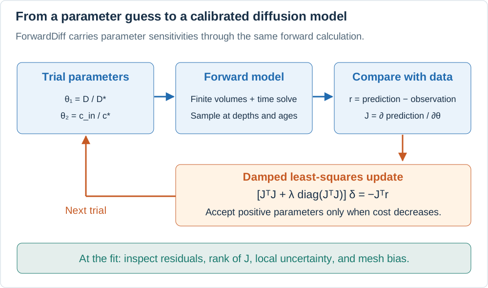
The loop reuses the same physical model at each trial parameter pair. Its sensitivities also support the later identifiability and uncertainty checks.

Set   . Equal independent noise variance makes ordinary least squares appropriate. With different known standard deviations, use and scale the Jacobian rows likewise; correlated errors require a corresponding covariance weighting.

Linearize around the current estimate:    . Minimizing the squared length of this approximation gives the Gauss–Newton normal equations

Levenberg–Marquardt adds damping to control the trial step. The implementation below uses diagonal scaling, specifically

This is not  . For large the step approaches , a scaled negative-gradient direction. Small damping approaches Gauss–Newton. The code accepts a trial only if both parameters remain positive and the actual residual sum decreases. Success divides damping by three; failure multiplies it by five before another trial. Thus the small-step argument does not guarantee that an arbitrary trial will succeed.

The printed history stores  ; the factor two changes neither the minimizer nor the step. The starting diffusivity is three times the true value and the starting inlet concentration is 40% too low.

This compact solver is suitable for the two sensitive parameters shown here. A zero-sensitivity parameter such as porosity would leave a zero diagonal entry; this damping cannot repair that lack of information. The solver stops after a small cost change, a failed set of trials, or the iteration limit, without a separate convergence-status object. Inspect the cost history and residuals before treating its returned parameters as a successful calibration. A related material example is in Parameter identification.

function levenberg_marquardt(f, θ; λ = 1.0e-3, maxiter = 40)
    r = f(θ)
    cost = sum(abs2, r)
    history = [cost]
    for _ in 1:maxiter
        J = ForwardDiff.jacobian(f, θ)
        H = J' * J
        g = J' * r
        improved = false
        for _ in 1:30
            θ_new = θ .- (H + λ * Diagonal(diag(H))) \ g
            if all(>(0), θ_new)
                r_new = f(θ_new)
                cost_new = sum(abs2, r_new)
                if cost_new < cost
                    θ, r, cost = θ_new, r_new, cost_new
                    λ = max(λ / 3, 1.0e-12)
                    improved = true
                    break
                end
            end
            λ *= 5
        end
        push!(history, cost)
        improved || break
        abs(history[end - 1] - history[end]) < 1.0e-12 * history[end] && break
    end
    return θ, history, r
end

residual(θ) = simulate(θ) .- c_obs
θ_start = [3.0, 0.6]      # D three times too large, c_in 40 % too small
θ_fit, history, r_fit = levenberg_marquardt(residual, θ_start)

println("iteration   sum of squared residuals")
for (k, c) in enumerate(history)
    @printf("  %2d        %.6e\n", k - 1, c)
end

iteration   sum of squared residuals
   0        2.586589e-01
   1        1.065001e-01
   2        1.695061e-02
   3        5.238447e-04
   4        2.514766e-04
   5        2.507286e-04
   6        2.507284e-04
   7        2.507284e-04
   8        2.507284e-04

8. Interpret parameter uncertainty and the fitted profiles

Near a well-determined optimum, linearize the predictions using the fitted Jacobian. With independent, zero-mean, equal-variance noise and negligible model error, the local covariance estimate of the scaled parameters is:

with measurements and parameters. The square roots of its diagonal are the standard errors, and is the correlation between the two estimates. Here  ,  , and    residual degrees of freedom. To recover physical parameter covariance, use   with  . The printed standard error for therefore multiplies the scaled value by m²/s.

A standard error is a local estimate of sampling variability, not a guaranteed error bound or automatically a 95% confidence interval. Model mismatch, boundary uncertainty, and discretization bias are not included. Poor rank or severe nonlinearity can make this approximation unreliable.

J_fit = ForwardDiff.jacobian(simulate, θ_fit)
σ²_hat = sum(abs2, r_fit) / (length(c_obs) - length(θ_fit))
Σ = σ²_hat * inv(Symmetric(J_fit' * J_fit))
standard_error = sqrt.(diag(Σ))
correlation = Σ[1, 2] / (standard_error[1] * standard_error[2])

@printf("estimated noise: %.4f mol/m³ (true value %.4f)\n\n", sqrt(σ²_hat), SIGMA)
println("parameter        true          start         identified     standard error")
@printf("D [m²/s]         %.4e    %.4e    %.4e     ± %.1e\n", D_TRUE, θ_start[1] * 1.0e-10, θ_fit[1] * 1.0e-10, standard_error[1] * 1.0e-10)
@printf("c_in [mol/m³]    %.4f        %.4f        %.4f         ± %.1e\n", C_IN_TRUE, θ_start[2], θ_fit[2], standard_error[2])
@printf("\ncorrelation between D and c_in: %+.2f\n", correlation)

estimated noise: 0.0050 mol/m³ (true value 0.0050)

parameter        true          start         identified     standard error
D [m²/s]         1.0000e-10    3.0000e-10    1.0164e-10     ± 1.3e-12
c_in [mol/m³]    1.0000        0.6000        0.9991         ± 4.4e-03

correlation between D and c_in: -0.69

Starting three times too high, is recovered to 1.6 %, and to 0.1 %. The estimated noise matches the one that was added. Both identified values lie within 1.3 standard errors of the values used to generate the data, as expected when the residuals are noise. These figures describe the seeded run and can shift with dependency versions. The uncertainty calculation requires one additional Jacobian evaluation at the fitted parameters, performed explicitly above.

The correlation is negative: a slightly larger spreads the profile, and a slightly smaller brings its level back down, so the two errors partly compensate. The plot shows the starting profiles as dotted curves and fitted profiles as solid curves. The vertical bars are   measurement-noise bars, not confidence bands for the fitted model or its parameters.

x, tsol_fit = solve_profiles(θ_fit[1] * 1.0e-10, θ_fit[2])
_, tsol_start = solve_profiles(θ_start[1] * 1.0e-10, θ_start[2])

p = plot(;
    xlabel = "depth x [m]", ylabel = "concentration c [mol/m³]",
    xlims = (0, 0.4), legend = :topright, size = (720, 440),
)
for (n, (t, color)) in enumerate(zip(T_OBS, (:steelblue, :darkorange)))
    label_t = @sprintf("t = %.0e s", t)
    plot!(p, x, tsol_start[1, :, n]; ls = :dot, color, label = "start, " * label_t)
    plot!(p, x, tsol_fit[1, :, n]; lw = 2, color, label = "identified, " * label_t)
    i = (n - 1) * length(X_OBS) .+ eachindex(X_OBS)
    scatter!(p, X_OBS, c_obs[i]; yerror = 2 * SIGMA, color, ms = 5, label = "measurements, " * label_t)
end
p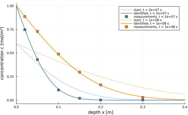

9. Separate numerical bias from measurement noise

The standard errors above account for measurement noise, and for nothing else. The fitted model also carries a discretization error, which biases the identified values whatever the quality of the data.

To isolate it, the model is fitted to the exact analytical values, without noise, on three grids. The remaining parameter difference combines spatial and temporal errors, optimizer termination error, and the finite-domain approximation to the semi-infinite reference. Here the far-boundary effect is negligible at the sampled points; the refinement trend tests whether spatial error dominates the others. Gauss–Newton starts from the calibrated values.

function fit_exact(N; θ = copy(θ_fit))
    f = θ -> simulate(θ; N) .- c_exact
    for _ in 1:10
        δ = -(ForwardDiff.jacobian(f, θ) \ f(θ))
        θ = θ .+ δ
        norm(δ) < 1.0e-10 && break
    end
    return θ
end

println("  N cells   h [mm]   relative bias on D   relative bias on c_in")
bias = map((100, 200, 400)) do N
    θ = fit_exact(N)
    @printf("  %4d      %4.1f      %+.3e           %+.3e\n", N, 1.0e3 * L / N, θ[1] - 1, θ[2] - 1)
    θ[1] - 1
end
@printf("\nrelative standard error on D from the noisy calibration: %.1e\n", standard_error[1] / θ_fit[1])

  N cells   h [mm]   relative bias on D   relative bias on c_in
   100      10.0      -9.075e-04           +3.069e-04
   200       5.0      -2.266e-04           +7.618e-05
   400       2.5      -5.689e-05           +1.862e-05

relative standard error on D from the noisy calibration: 1.3e-02

The bias is divided by about four each time the grid is refined by two: the scheme is second order in in this regime, and the parameter bias follows that trend. This interpretation depends on keeping observation points aligned and time and optimization errors small; it need not persist under unlimited mesh refinement.

On the default grid, the bias on is small compared with the standard error caused by the noise, so the grid is fine enough for these measurements. More precise measurements would shrink the standard error but not the bias, and the grid would then have to be refined until the bias is small compared with the standard error. A standard error smaller than the discretization bias gives a false sense of precision.

10. Checks and short exercises

• Units and storage: at   and   mol/m³, one cubic meter of material stores 0.30 mol. Explain why measuring that amount can reveal porosity even when measuring pore-solution concentration alone cannot in this model.

• Parameter scaling: a fitted   means    m²/s. A scaled standard error of 0.01 means m²/s. Verify the corresponding covariance transformation.

• Identifiability: retain only the first measurement row of J_ad. Its rank is at most one, so it cannot locally determine two parameters. Compare with rows spanning several depths and both ages; consider their sensitivity relative to noise, not just whether a singular value is mathematically nonzero.

• Derivative checks: vary the central-difference step over several decades, and tighten abstol and reltol in solve_profiles. Compare absolute errors at low-concentration points and repeat the linearity check for .

• Numerical bias: compare the 100-, 200-, and 400-interval fits at the same depths and ages. Halving the mesh spacing should reduce the leading spatial bias by about four until other errors dominate. A small least-squares residual by itself does not establish accuracy of the identified diffusivity.

• Experimental assumptions: what changes if the inlet varies with time, the solute binds to the solid, or measurements are slice averages? Adjust the forward model and measurement operator before interpreting the fitted physically.

The conceptual illustrations can be regenerated with python3 examples/fickian_identification/draw_schematics.py.