Cryer's Problem

A saturated poroelastic sphere, drained at its surface, loaded at   by a uniform radial compression. The pore pressure at the centre rises 23 % above its undrained value before decaying — the Mandel–Cryer effect (Cryer, 1963), three times stronger here than in the plane-strain Mandel case, which makes this the most severe of the three poroelastic benchmarks.

It is also the case that forces a curvilinear element. Terzaghi and Mandel are Cartesian; spherical symmetry brings in hoop strains   that no Cartesian element produces, and an integration weight. The element written below is the prototype of the axisymmetric machinery the Barcelona Basic Model will need.

Problem

Sphere of radius . At   a compressive radial traction is applied to the surface, which is held drained.

Boundary	Condition
	symmetry:  , no flux
	drained  , traction

Reference solution

Derived here rather than transcribed, from the single-porosity formulation of (Mehrabian and Abousleiman, 2018) (their Table 1). Spherical symmetry makes the displacement field irrotational, so the momentum balance integrates once to

with an unknown function of time alone. Substituting into the fluid mass balance leaves a diffusion equation for the pressure with a source driven by :

is exactly the storage coefficient the package already uses:   is the same consolidation coefficient as in the Terzaghi and Mandel benchmarks.

In Laplace space this is an ordinary differential equation. Taking the solution regular at  , imposing  , integrating    and closing with the traction condition    gives, in   and   with conjugate to :

with  . The inversion to the time domain is numerical, by the Stehfest algorithm — the same route the source paper takes.

The expression is checked by the initial and final value theorems before it is used: it must give the Skempton response  , uniform in , and decay to zero.

include("biot_common.jl")

uniform_schedule (generic function with 1 method)

Model

The same material as Mandel's problem, so the two spherical and plane-strain overshoots are directly comparable.

const CRYER_MATERIAL = HomogeneousBiot(;
    E = 1.0e8, nu = 0.2, k = 1.0e-13, mu_l = 1.0e-3, b = 1.0, N = 7.2e-9,
)

const R_SPHERE = 1.0    # radius [m]
const P_CONF = 1.0e6    # confining traction [Pa]

# `compaction_coefficient` and `storage_coefficient` come from the package.

1.0e6

Reference solution in Laplace space

sinh(√ŝ) overflows above ŝ ≈ 1e5, so both quotients are written in forms that stay finite: the ratio as decaying exponentials, and g(x)/(x² sinh x) as coth(x)/x − 1/x².

_shape_ratio(r, x) = exp((r - 1) * x) * (1 - exp(-2r * x)) / (r * (1 - exp(-2x)))
_g_term(x) = coth(x) / x - 1 / x^2

"""
    cryer_laplace(m, r, ŝ; Pc) -> P̃(r*, ŝ)

Pore pressure in Laplace space, with `ŝ` conjugate to the dimensionless time `t* = ct/R²`.
"""
function cryer_laplace(m::HomogeneousBiot, r, ŝ; Pc = P_CONF)
    _, G = lame(m)
    S = storage_coefficient(m)
    q = m.b * compaction_coefficient(m) / S
    x = sqrt(ŝ)
    D = (1 + m.nu) / (3 * (1 - 2m.nu)) + 2q / 3 - 2q * _g_term(x)
    return (Pc / ŝ) * (m.b / (2G * S)) * (1 - _shape_ratio(r, x)) / D
end

cryer_laplace (generic function with 1 method)

Inversion

By the Stehfest algorithm of biot_common.jl. This transform is elementary, so it evaluates in BigFloat throughout.

"""
    cryer_pressure(m, r, t; Pc) -> p [Pa]

Pore pressure at normalised radius `r = r/R` and dimensionless time `t = c t/R²`.
"""
function cryer_pressure(m::HomogeneousBiot, r, t; Pc = P_CONF)
    t <= 0 && return skempton(m) * Pc
    return stehfest(ŝ -> cryer_laplace(m, big(r), ŝ; Pc = Pc), t)
end

cryer_pressure (generic function with 1 method)

The spherical element

This is the part Terzaghi and Mandel did not need. In spherical symmetry the strain has three non-zero normal components,

so the discrete strain operator for shape function is       and the volume element carries . Contracting with the isotropic stiffness gives, for the mechanical block,

The hoop terms are what a Cartesian element cannot produce. The element itself lives in benchmarks/biot_common.jl as radial_element_matrices!, parameterised by the number of hoop directions: nhoop = 2 here, nhoop = 1 for the cylinder of de Leeuw's problem.

Solving

"""
    run_cryer(; m, nel, T_probe, T_start, dT)

Return `(m, r, T_probe, profiles, T_hist, p_centre)`.
"""
function run_cryer(;
        m = CRYER_MATERIAL,
        nel = 80,
        T_probe = [0.01, 0.03, 0.06, 0.1, 0.2, 0.5],
        T_start = 1.0e-4,
        dT = 5.0e-4,
    )
    c = consolidation_coefficient(m)
    t_of_T(T) = T * R_SPHERE^2 / c

    grid = generate_grid(Line, (nel,), Vec(0.0), Vec(R_SPHERE))

    ip = Lagrange{RefLine, 1}()
    dh = DofHandler(grid)
    add!(dh, :u, ip)
    add!(dh, :p, ip)
    close!(dh)

    qr = QuadratureRule{RefLine}(2)
    cv_u = CellValues(qr, ip, ip)
    cv_p = CellValues(qr, ip, ip)

    # Symmetry at the centre, drainage at the surface
    ch = ConstraintHandler(dh)
    add!(ch, Dirichlet(:u, getfacetset(grid, "left"), (x, t) -> 0.0))
    add!(ch, Dirichlet(:p, getfacetset(grid, "right"), (x, t) -> 0.0))
    close!(ch)
    update!(ch, 0.0)

    n_loc = ndofs_per_cell(dh)
    K1 = allocate_matrix(dh)
    K2 = allocate_matrix(dh)
    A = allocate_matrix(dh)
    as1 = start_assemble(K1)
    as2 = start_assemble(K2)
    ke1 = zeros(n_loc, n_loc)
    ke2 = zeros(n_loc, n_loc)

    for cell in CellIterator(dh)
        reinit!(cv_u, cell)
        reinit!(cv_p, cell)
        radial_element_matrices!(ke1, ke2, m, cv_u, cv_p, getcoordinates(cell); nhoop = 2)
        assemble!(as1, celldofs(cell), ke1)
        assemble!(as2, celldofs(cell), ke2)
    end

    # Node → dof maps (scalar u in 1D, so one dof per node per field)
    u_dof = zeros(Int, getnnodes(grid))
    p_dof = zeros(Int, getnnodes(grid))
    u_range = dof_range(dh, :u)
    p_range = dof_range(dh, :p)
    for cell in CellIterator(dh)
        d = celldofs(cell)
        for (loc, node) in enumerate(cell.nodes)
            u_dof[node] = d[u_range[loc]]
            p_dof[node] = d[p_range[loc]]
        end
    end

    # Surface traction: the boundary term of the weak form is δu σ_rr r², evaluated at
    # r = R where σ_rr = −P_c.
    coords = [node.x[1] for node in grid.nodes]
    surface_node = argmax(coords)
    f_ext = zeros(ndofs(dh))
    f_ext[u_dof[surface_node]] = -P_CONF * R_SPHERE^2

    schedule = uniform_schedule(T_probe; T_start = T_start, dT = dT)

    x = zeros(ndofs(dh))
    apply!(x, ch)

    profiles = Vector{Vector{Float64}}()
    probes_left = sort(T_probe)
    T_hist = Float64[]
    p_centre = Float64[]
    centre_node = argmin(coords)
    t_prev = 0.0

    for T in schedule
        t = t_of_T(T)
        dt = t - t_prev
        combine!(A, K1, K2, 1.0 / dt)
        rhs = copy(f_ext)
        mul!(rhs, K2, x, 1.0 / dt, 1.0)
        apply!(A, rhs, ch)
        x = A \ rhs
        t_prev = t

        push!(T_hist, T)
        push!(p_centre, x[p_dof[centre_node]])

        if !isempty(probes_left) && isapprox(T, probes_left[1]; rtol = 1.0e-9)
            push!(profiles, [x[p_dof[i]] for i in 1:getnnodes(grid)])
            popfirst!(probes_left)
        end
    end

    return m, coords, sort(T_probe), profiles, T_hist, p_centre
end

model, rr, T_probe, p_num, T_hist, p_centre = run_cryer()

(BiotPoroelastic{Float64}(1.0e8, 0.2, 1.0e-13, 0.001, 1.0, 7.2e-9), [0.0, 0.012500000000000011, 0.025000000000000022, 0.03749999999999998, 0.04999999999999999, 0.0625, 0.07500000000000001, 0.08750000000000002, 0.09999999999999998, 0.11249999999999999  …  0.8875, 0.9, 0.9125, 0.925, 0.9375, 0.95, 0.9625, 0.975, 0.9875, 1.0], [0.01, 0.03, 0.06, 0.1, 0.2, 0.5], [[800003.2206950323, 800003.2192483153, 800003.2160303295, 800003.2105762335, 800003.2023894881, 800003.1907720919, 800003.1747411056, 800003.1529346193, 800003.1234869849, 800003.0838600121  …  432854.24834182946, 391036.1122396604, 346940.30918316735, 300808.76582433784, 252930.75433375748, 203637.78936851557, 153296.75709736775, 102301.50518044019, 51063.220322852496, 0.0], [860148.0521138081, 860134.27877389, 860104.5463724758, 860056.5093525266, 859988.9827641146, 859900.7500537421, 859790.3561865925, 859656.0426663462, 859495.7114159899, 859306.8952322381  …  255276.30715822705, 227221.36100469608, 198924.3497869783, 170454.45054378445, 141882.34172599053, 113279.67458306621, 84718.53087958103, 56270.87399047583, 28008.000569908658, 0.0], [860695.3740305046, 860557.8133199579, 860262.6822020645, 859790.5777234272, 859136.0719251712, 858295.985072367, 857267.4700691025, 856047.5361175842, 854632.8906547523, 853019.8796500966  …  169720.98003924135, 150525.54831913902, 131360.2878638771, 112248.67135602137, 93214.094821535, 74279.79515077814, 55468.76842146663, 36803.689534403, 18306.83366262176, 0.0], [723023.6638140382, 722818.8247266064, 722379.8802134282, 721679.1002836978, 720710.230882251, 719471.0538522392, 717960.5360965709, 716178.1164561367, 714123.4633497088, 711796.3764477542  …  116617.94496182076, 103300.75888124749, 90050.03532046218, 76876.01242055955, 63788.82029504307, 50798.46242365841, 37914.797387015795, 25147.52100994663, 12506.148979354119, 0.0], [365127.08321780723, 365004.31911807833, 364741.3331867016, 364321.68641413137, 363741.9133916338, 363001.07286979904, 362099.03848026105, 361036.06954495277, 359812.66330025205, 358429.49285775586  …  54196.176510767444, 47983.48819159562, 41810.2308879258, 35680.0391298339, 29596.49634209732, 23563.131951412342, 17583.418552088853, 11660.769133669663, 5798.534373855832, 0.0], [40750.08571105476, 40736.27025315666, 40706.67512494313, 40659.45126045644, 40594.210125729056, 40510.847787397695, 40409.35255205027, 40289.75665657631, 40152.119624163075, 39996.521265675685  …  6021.3837354871275, 5330.986257088995, 4645.022309686484, 3963.888765682414, 3287.9768216631765, 2617.6717113058307, 1953.3524241309847, 1295.3914303191336, 644.154411824016, 0.0]], [0.0001, 0.0006000000000000001, 0.0011, 0.0016, 0.0021, 0.0026, 0.0031, 0.0036, 0.0041, 0.0046  …  0.4956, 0.4961, 0.4966, 0.4971, 0.4976, 0.4981, 0.4986, 0.4991, 0.4996, 0.5], [722131.616949284, 733823.1808950943, 741551.138649562, 747637.8121655141, 752802.2099091302, 757361.3804915139, 761485.5484977256, 765277.9854336428, 768806.7379772216, 772119.3857367132  …  42083.595670918956, 41929.89413181136, 41776.75395173522, 41624.1730805475, 41472.14947556515, 41320.681101553906, 41169.76593077603, 41019.40194279619, 40869.587124625104, 40750.08571105476])

Results

using Plots

B = skempton(model)
p0 = B * P_CONF

@printf("Skempton B         : %.6f\n", B)
@printf("Undrained p₀ = B·P_c: %.4e Pa\n", p0)
@printf("Storage S          : %.4e Pa⁻¹\n", storage_coefficient(model))
@printf("Diffusivity c      : %.4e m²/s\n", consolidation_coefficient(model))
println()

Skempton B         : 0.714286
Undrained p₀ = B·P_c: 7.1429e+05 Pa
Storage S          : 1.6200e-08 Pa⁻¹
Diffusivity c      : 6.1728e-03 m²/s

The reference solution, checked before it is used

The Laplace expression must reproduce the Skempton response at  , uniformly in , and vanish at the drained surface.

@printf("p(r,t→0)/P_c at r* = 0.1, 0.5, 0.9 : %.6f  %.6f  %.6f   (B = %.6f)\n",
    cryer_pressure(model, 0.1, 1.0e-6) / P_CONF,
    cryer_pressure(model, 0.5, 1.0e-6) / P_CONF,
    cryer_pressure(model, 0.9, 1.0e-6) / P_CONF, B)
@printf("p at the drained surface, t* = 0.1 : %.3e Pa\n",
    cryer_pressure(model, 0.999999, 0.1))
println()

p(r,t→0)/P_c at r* = 0.1, 0.5, 0.9 : 0.715149  0.715149  0.715149   (B = 0.714286)
p at the drained surface, t* = 0.1 : 9.923e-01 Pa

The Mandel–Cryer overshoot

The discriminating quantity, and much larger here than in plane strain.

p_ref_centre = [cryer_pressure(model, 1.0e-8, T) for T in T_hist]

i_num = argmax(p_centre)
i_ref = argmax(p_ref_centre)
@printf("numerical peak : p/p₀ = %.5f at T = %.4f\n", p_centre[i_num] / p0, T_hist[i_num])
@printf("reference peak : p/p₀ = %.5f at T = %.4f\n", p_ref_centre[i_ref] / p0, T_hist[i_ref])
@printf("overshoot      : %.1f %% above p₀   (Mandel, plane strain: 6.5 %%)\n",
    100 * (p_ref_centre[i_ref] / p0 - 1))
println()

plt_hist = plot(
    T_hist, p_ref_centre ./ p0;
    xlabel = "T = c t / R²  [-]", ylabel = "p(0, t) / p₀  [-]",
    title = "Mandel–Cryer effect at the centre of the sphere",
    label = "reference (Laplace + Stehfest)", lw = 2, color = :black,
    xscale = :log10, legend = :bottomleft, size = (700, 420),
)
plot!(
    plt_hist, T_hist[1:8:end], (p_centre ./ p0)[1:8:end];
    seriestype = :scatter, ms = 3, mswidth = 0, color = :crimson, label = "finite elements",
)
hline!(plt_hist, [1.0]; ls = :dash, color = :grey, label = "p₀ = B·P_c")
plt_hist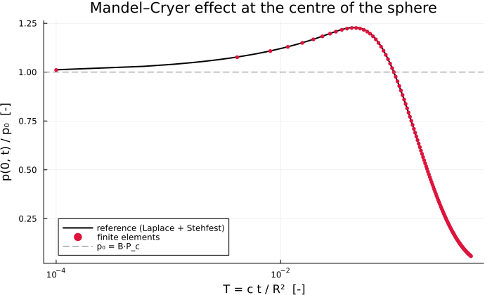

Error against the reference

println("      T     |  L2 error  |  L∞ error [Pa]")
println("-"^44)
errors = Float64[]
for (T, pn) in zip(T_probe, p_num)
    ref = [cryer_pressure(model, max(r / R_SPHERE, 1.0e-8), T) for r in rr]
    e2 = norm(pn .- ref) / norm(ref)
    push!(errors, e2)
    @printf("  %8.4f  |  %.3e |  %10.1f\n", T, e2, maximum(abs.(pn .- ref)))
end
println("-"^44)
@printf("worst relative L2 error: %.3e\n", maximum(errors))

      T     |  L2 error  |  L∞ error [Pa]
--------------------------------------------
    0.0100  |  2.667e-03 |      4986.9
    0.0300  |  1.621e-03 |      1767.2
    0.0600  |  1.408e-03 |      1476.1
    0.1000  |  8.372e-04 |       680.7
    0.2000  |  2.696e-03 |      1085.3
    0.5000  |  6.621e-03 |       272.1
--------------------------------------------
worst relative L2 error: 6.621e-03

Convergence

function worst_error(; nel, dT)
    mm, rrr, Tp, pn, _, _ = run_cryer(; nel = nel, dT = dT)
    return maximum(
        let ref = [cryer_pressure(mm, max(r / R_SPHERE, 1.0e-8), T) for r in rrr]
            norm(p .- ref) / norm(ref)
        end for (T, p) in zip(Tp, pn)
    )
end

worst_error (generic function with 1 method)

Halving halves the error — backward Euler, first order in time.

println("  ΔT        |  worst L2 error |  ratio")
println("-"^42)
prev = NaN
for dT in (4.0e-3, 2.0e-3, 1.0e-3, 5.0e-4)
    e = worst_error(; nel = 80, dT = dT)
    @printf("  %.2e  |    %.3e    |  %s\n", dT, e, isnan(prev) ? "—" : @sprintf("%.2f", prev / e))
    global prev = e
end

  ΔT        |  worst L2 error |  ratio
------------------------------------------
  4.00e-03  |    5.351e-02    |  —
  2.00e-03  |    2.682e-02    |  2.00
  1.00e-03  |    1.334e-02    |  2.01
  5.00e-04  |    6.621e-03    |  2.01

Refining the mesh at fixed changes almost nothing: the spatial error of the radial element is already well under the temporal floor by forty elements.

println("\n  elements  |  worst L2 error")
println("-"^32)
for n in (20, 40, 80, 160)
    @printf("  %8d  |    %.3e\n", n, worst_error(; nel = n, dT = 5.0e-4))
end

  elements  |  worst L2 error
--------------------------------
        20  |    7.225e-03
        40  |    6.714e-03
        80  |    6.621e-03
       160  |    6.602e-03

Radial profiles

plt = plot(;
    xlabel = "r / R  [-]", ylabel = "p / p₀  [-]",
    title = "Cryer — radial pressure profiles",
    legend = :bottomleft, size = (700, 440),
)
rfine = range(0.001, 0.999; length = 200)
palette = cgrad(:viridis, max(length(T_probe), 2); categorical = true)
for (i, (T, pn)) in enumerate(zip(T_probe, p_num))
    plot!(
        plt, rfine, [cryer_pressure(model, r, T) / p0 for r in rfine];
        color = palette[i], lw = 2, label = "T = $T",
    )
    plot!(
        plt, rr ./ R_SPHERE, pn ./ p0;
        color = palette[i], seriestype = :scatter, ms = 2, mswidth = 0, label = "",
    )
end
plt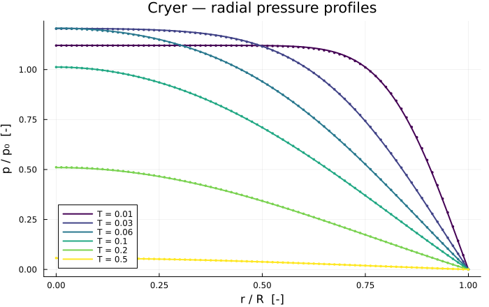

Notes

• The element is the new part — hoop strains and an weight. It is written out by hand here; the same kinematics, in cylindrical coordinates, is what the Barcelona Basic Model will need for axisymmetry.

• BigFloat for the Stehfest weights is not optional: they alternate in sign and grow to , and in Float64 the cancellation leaves nothing.

• The reference is derived, not transcribed. The published closed-form series for this problem could not be reproduced from the printed prefactor; deriving the Laplace solution and inverting it numerically avoids the question entirely, and the initial and final value theorems check it independently.