
Terzaghi 1D Consolidation
The canonical verification of a poroelastic solver: a saturated column, laterally confined, drained at the top, loaded instantaneously. Terzaghi's closed-form series gives the excess pore pressure at every depth and time, so the numerical solution can be checked against an exact answer rather than against another code (Terzaghi, 1943).
Problem
A column of height
The one-dimensional Biot equations reduce to
with
Reference solution
With
The two constants follow from the equations above — the consolidation coefficient from eliminating
At
include("biot_common.jl")uniform_schedule (generic function with 1 method)Model
The material is the shared HomogeneousBiot of benchmarks/biot_common.jl; the geometry and the load belong to this benchmark.
const TERZAGHI_MATERIAL = HomogeneousBiot(;
    E = 1.0e7, nu = 0.2, k = 1.0e-13, mu_l = 1.0e-3, b = 1.0, N = 1.0e-10,
)

const H = 1.0        # column height [m]
const W = 0.1        # column width [m] — immaterial, the column is laterally confined
const F_LOAD = 1.0e4 # surface load [Pa]

"""Initial (undrained) excess pore pressure ``p_0 = F b / (M_o N + b^2)`` [Pa]."""
initial_pressure(m::HomogeneousBiot, F = F_LOAD) =
    F * m.b / (oedometric_modulus(m) * m.N + m.b^2)
initial_pressure (generic function with 2 methods)Reference series
"""
    terzaghi_pressure(Z, T; nterms = 400)

Excess pore pressure `p/p₀` at normalized depth `Z = (H-y)/H` below the drained surface
and dimensionless time `T = c_v t / H²`.

The series converges slowly for small `T` — the terms decay like `exp(-(2m+1)²π²T/4)` — so
`nterms` is generous by default; the summation cost is negligible next to the solve.
"""
function terzaghi_pressure(Z, T; nterms = 400)
    T <= 0 && return 1.0
    s = 0.0
    for m in 0:(nterms - 1)
        a = (2m + 1) * π / 2
        s += (2 / a) * sin(a * Z) * exp(-a^2 * T)
    end
    return s
end

"""Downward traction `-F_LOAD` on the loaded top facet."""
function PoroMechanics.facet_load!(fe, facet, m::HomogeneousBiot, fv_u)
    fill!(fe, 0.0)
    reinit!(fv_u, facet)
    for q in 1:getnquadpoints(fv_u)
        dΓ = getdetJdV(fv_u, q)
        traction = Vec{2}((0.0, -F_LOAD))
        for i in 1:getnbasefunctions(fv_u)
            fe[i] += (shape_value(fv_u, q, i) ⋅ traction) * dΓ
        end
    end
    return nothing
end
Solving
One short step to T_start captures the undrained response — the load produces
"""
    run_terzaghi(; m, nely, T_probe, T_start)

Solve the column and return `(m, y, times, pressures)` where `pressures[i]` is the
pressure profile sampled at the nodes of `y` at dimensionless time `T_probe[i]`.
"""
function run_terzaghi(;
        m = TERZAGHI_MATERIAL,
        nely = 60,
        T_probe = [0.01, 0.05, 0.1, 0.2, 0.5, 1.0],
        T_start = 1.0e-4,
        dT = 2.5e-4,
    )
    c_v = consolidation_coefficient(m)
    t_of_T(T) = T * H^2 / c_v

    grid = generate_grid(Quadrilateral, (1, nely), Vec(0.0, 0.0), Vec(W, H))

    ip_geo = Lagrange{RefQuadrilateral, 1}()
    ip_u = Lagrange{RefQuadrilateral, 1}()^2
    ip_p = Lagrange{RefQuadrilateral, 1}()

    dh = DofHandler(grid)
    add!(dh, :u, ip_u)
    add!(dh, :p, ip_p)
    close!(dh)

    qr = QuadratureRule{RefQuadrilateral}(2)
    qr_fac = FacetQuadratureRule{RefQuadrilateral}(2)
    cv_u = CellValues(qr, ip_u, ip_geo)
    cv_p = CellValues(qr, ip_p, ip_geo)
    fv_u = FacetValues(qr_fac, ip_u, ip_geo)

    # Drained top, rollers on the sides, clamped base.
    ch = ConstraintHandler(dh)
    add!(ch, Dirichlet(:p, getfacetset(grid, "top"), (x, t) -> 0.0))
    add!(ch, Dirichlet(:u, getfacetset(grid, "left"), (x, t) -> 0.0, [1]))
    add!(ch, Dirichlet(:u, getfacetset(grid, "right"), (x, t) -> 0.0, [1]))
    add!(ch, Dirichlet(:u, getfacetset(grid, "bottom"), (x, t) -> 0.0, [2]))
    close!(ch)
    update!(ch, 0.0)

    K1, K2 = assemble_biot_matrices(dh, cv_u, cv_p, m; constraints = ch)
    f_ext = assemble_biot_load(dh, getfacetset(grid, "top"), fv_u, m)

    coords = [node.x for node in grid.nodes]
    y = [c[2] for c in coords]
    p_dof = node_dof_maps(dh, grid, :p).p

    # One short step to T_start captures the undrained response, then uniform steps.
    # Backward Euler is first order in time, so ΔT — not the number of steps — sets the
    # temporal error; it must be small enough not to mask the spatial error.
    schedule = uniform_schedule(T_probe; T_start = T_start, dT = dT)

    pressures = Vector{Vector{Float64}}()
    probes_left = sort(T_probe)
    function save_probe(x, t, step)
        T = schedule[step]
        if !isempty(probes_left) && isapprox(T, probes_left[1]; rtol = 1.0e-9)
            push!(pressures, x[p_dof])
            popfirst!(probes_left)
        end
    end
    solve_biot(K1, K2, ch;
        inival = zeros(ndofs(dh)), times = vcat(0.0, t_of_T.(schedule)),
        load = f_ext, on_step = save_probe,
    )

    return m, y, sort(T_probe), pressures
end

model, y, T_probe, p_num = run_terzaghi()
(BiotPoroelastic{Float64}(1.0e7, 0.2, 1.0e-13, 0.001, 1.0, 1.0e-10), [0.0, 0.0, 0.016666666666666663, 0.016666666666666663, 0.033333333333333326, 0.033333333333333326, 0.04999999999999999, 0.04999999999999999, 0.06666666666666665, 0.06666666666666665 … 0.9333333333333333, 0.9333333333333333, 0.95, 0.95, 0.9666666666666667, 0.9666666666666667, 0.9833333333333333, 0.9833333333333333, 1.0, 1.0], [0.01, 0.05, 0.1, 0.2, 0.5, 1.0], [[9988.901220057745, 9988.901220057764, 9988.90121988253, 9988.901219882544, 9988.901219285686, 9988.901219285703, 9988.901218026871, 9988.901218026896, 9988.901215606998, 9988.901215607024 … 3648.4254278099365, 3648.425427809935, 2781.166539557627, 2781.1665395576365, 1876.026548399497, 1876.0265483994967, 944.7028140404539, 944.7028140404599, 0.0, 0.0], [9956.858101611602, 9956.858101611619, 9956.38441014634, 9956.384410146362, 9954.954241717285, 9954.9542417173, 9952.540259568486, 9952.540259568494, 9949.096721780936, 9949.096721780934 … 1670.5200407767913, 1670.5200407767459, 1256.9606982453238, 1256.9606982452992, 839.9219970757656, 839.9219970757256, 420.5474248643332, 420.54742486429836, 0.0, 0.0], [9482.050609626833, 9482.050609626873, 9480.023274873909, 9480.023274873945, 9473.935615932567, 9473.935615932602, 9463.770707768936, 9463.770707768977, 9449.500471935047, 9449.500471935073 … 1184.5462717256298, 1184.546271725816, 889.8538889204765, 889.8538889206237, 593.9253425836789, 593.92534258375, 297.1698390454767, 297.16983904547897, 0.0, 0.0], [7715.734589656467, 7715.734589656469, 7713.228544029136, 7713.228544029133, 7705.711275262571, 7705.711275262571, 7693.185392326712, 7693.185392326724, 7675.655258881883, 7675.655258881897 … 827.3530920734001, 827.3530920736072, 621.0869905449662, 621.0869905451074, 414.3307021458912, 414.3307021459681, 207.24721284612227, 207.24721284612076, 0.0, 0.0], [3704.966513730593, 3704.9665137305915, 3703.6970928008095, 3703.6970928008036, 3699.889698908265, 3699.889698908259, 3693.546938154669, 3693.5469381546777, 3684.673152080887, 3684.673152080901 … 387.30140623759564, 387.3014062379183, 290.7086486864733, 290.70864868668025, 193.91657058034292, 193.91657058029975, 96.99153587686162, 96.99153587677604, 0.0, 0.0], [1079.211561931507, 1079.211561931556, 1078.8417430858872, 1078.8417430859338, 1077.7325400043683, 1077.7325400044142, 1075.884712879299, 1075.8847128793332, 1073.299528118985, 1073.2995281190197 … 112.80832652342222, 112.8083265232141, 84.67396356042444, 84.67396356037304, 56.481569291031235, 56.48156929125895, 28.250465374650584, 28.250465374764747, 0.0, 0.0]])Comparison with the reference solution
using Plots

p0 = initial_pressure(model)
c_v = consolidation_coefficient(model)

@printf("Oedometric modulus M_o : %.4e Pa\n", oedometric_modulus(model))
@printf("Consolidation coeff c_v: %.4e m²/s\n", c_v)
@printf("Undrained pressure p₀  : %.4e Pa  (load F = %.1e Pa)\n", p0, F_LOAD)
println()

Z = (H .- y) ./ H

"""Relative L2 error of a numerical profile against the reference series."""
function l2_error(pnum, T)
    ref = [terzaghi_pressure(z, T) * p0 for z in Z]
    return norm(pnum .- ref) / norm(ref)
end

println("      T     |  L2 error  |  L∞ error [Pa]")
println("-"^44)
errors = Float64[]
for (T, pn) in zip(T_probe, p_num)
    ref = [terzaghi_pressure(z, T) * p0 for z in Z]
    e2 = norm(pn .- ref) / norm(ref)
    einf = maximum(abs.(pn .- ref))
    push!(errors, e2)
    @printf("  %8.4f  |  %.3e |  %10.3f\n", T, e2, einf)
end
println("-"^44)
@printf("worst relative L2 error: %.3e\n", maximum(errors))
Oedometric modulus M_o : 1.1111e+07 Pa
Consolidation coeff c_v: 1.1099e-03 m²/s
Undrained pressure p₀ : 9.9889e+03 Pa (load F = 1.0e+04 Pa)
T | L2 error | L∞ error [Pa]
--------------------------------------------
0.0100 | 1.240e-03 | 31.821
0.0500 | 4.275e-04 | 6.412
0.1000 | 2.765e-04 | 3.149
0.2000 | 2.162e-04 | 1.467
0.5000 | 3.533e-04 | 1.307
1.0000 | 5.929e-04 | 0.640
--------------------------------------------
worst relative L2 error: 1.240e-03Convergence
A single error figure proves little — it could hide a compensating pair of mistakes. What a benchmark has to show is that the error goes to zero at the expected rate.
function worst_error(; nely, dT)
    mm, yy, Tp, pn = run_terzaghi(; nely = nely, dT = dT)
    q0 = initial_pressure(mm)
    ZZ = (H .- yy) ./ H
    return maximum(
        let ref = [terzaghi_pressure(z, T) * q0 for z in ZZ]
            norm(pv .- ref) / norm(ref)
        end for (T, pv) in zip(Tp, pn)
    )
end
worst_error (generic function with 1 method)Halving
println("  ΔT        |  worst L2 error |  ratio")
println("-"^42)
prev = NaN
for dT in (2.0e-3, 1.0e-3, 5.0e-4, 2.5e-4)
    e = worst_error(; nely = 60, dT = dT)
    @printf("  %.2e  |    %.3e    |  %s\n", dT, e, isnan(prev) ? "—" : @sprintf("%.2f", prev / e))
    global prev = e
end
ΔT | worst L2 error | ratio
------------------------------------------
2.00e-03 | 9.871e-03 | —
1.00e-03 | 4.996e-03 | 1.98
5.00e-04 | 2.494e-03 | 2.00
2.50e-04 | 1.240e-03 | 2.01Refining the mesh instead, at a fixed
println("\n  elements  |  worst L2 error")
println("-"^32)
for n in (15, 30, 60, 120)
    @printf("  %8d  |    %.3e\n", n, worst_error(; nely = n, dT = 2.5e-4))
end
  elements  |  worst L2 error
--------------------------------
        15  |    5.072e-03
        30  |    1.560e-03
        60  |    1.240e-03
       120  |    1.273e-03
Pressure profiles
Markers are the finite element solution, solid lines the Terzaghi series. The isochrones flatten as the pressure diffuses towards the drained surface at
plt = plot(;
    xlabel = "p / p₀  [-]",
    ylabel = "Z = (H − y) / H  [-]",
    title = "Terzaghi consolidation — numerical vs analytical",
    yflip = true,
    legend = :bottomleft,
    size = (700, 460),
)

Zfine = range(0, 1; length = 400)
order = sortperm(Z)
palette = cgrad(:viridis, max(length(T_probe), 2); categorical = true)

for (i, (T, pn)) in enumerate(zip(T_probe, p_num))
    plot!(
        plt, [terzaghi_pressure(z, T) for z in Zfine], Zfine;
        color = palette[i], lw = 2, label = "T = $T",
    )
    plot!(
        plt, (pn ./ p0)[order], Z[order];
        color = palette[i], seriestype = :scatter, ms = 3, mswidth = 0, label = "",
    )
end
plt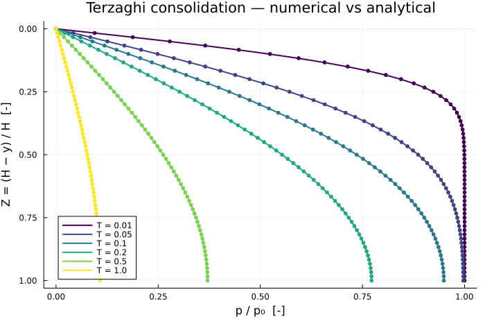
Notes
Equal-order elements —
and both P1. This is not inf-sup stable in general, but the Biot storage term The first step sets the initial condition — the column starts unloaded, and the load is applied over the first step. That step must be short enough that the column is still essentially undrained, so it produces
and not a partly dissipated pressure. Everything after it is marched with a uniform . Series truncation — the reference sum converges slowly at small
; 400 terms keeps the truncation error far below the discretization error being measured.