Fickian Diffusion 1D

Diffusion of a solute in a saturated porous medium, on VoronoiFVM.jl. This is the simplest model in the package: one species, a linear equation, and a closed-form reference solution — so it is the case that validates the whole AbstractPoroModel → closures → VoronoiFVM chain.

Physical problem

A solute diffuses into a saturated soil column. The concentration [mol/m³] is the only unknown, and it obeys

The porosity cancels, leaving pure diffusion:

Boundary	Condition
(inlet)	Dirichlet
(outlet)	Zero Neumann   (the VoronoiFVM default)

The initial condition is  , with   so that it is consistent with the boundary condition — see the note at the end of this page.

Reference solution

On a semi-infinite domain the solution is

valid as long as the diffusion front stays small compared with .

Parameters

Symbol	Value	Unit	Description
		—	Porosity
		m²/s	Effective diffusion coefficient
		mol/m³	Concentration imposed at the inlet
		m	Column length

The characteristic diffusion time is    s. The simulation covers   s , an early transient in which the front penetrates only about   m.

using PoroMechanics
using VoronoiFVM
using ExtendableGrids

The model

FickModel lives in the package, not in this script. Diffusion through a saturated medium is the same equation whatever column it is solved on; what belongs here is the material data, the geometry, and the concentration imposed at the inlet.

That imposed concentration is given as data — dirichlet = ((1, c_in),), meaning "impose c_in on boundary region 1" — rather than written into a method, so the same model serves a column fed from the other end without editing anything. The sealed face at   needs no code at all: zero flux is what VoronoiFVM does with a boundary nobody claims.

const C_IN = 1.0    # concentration imposed at x = 0 [mol/m³]

fick_material(; c_in = C_IN) = FickModel(;
    phi = 0.30,                  # porosity [-]
    D = 1.0e-10,                 # effective diffusion coefficient [m²/s]
    dirichlet = ((1, c_in),),    # imposed concentration at x = 0
)

fick_material (generic function with 1 method)

Solving

function run_fickian_diffusion(; L = 1.0, N = 100, t_end = 1e8, Δt0 = 1e4, n_save = 20)
    m = fick_material()

    # Uniform 1D grid
    grid = simplexgrid(range(0, L; length = N + 1))

    sys = fvm_system(m, grid)

    # Initial condition: zero concentration except at the Dirichlet node (x=0).
    # Without that consistency the time step controller sees Δu=1 at the first
    # step and shrinks Δt forever (Dirichlet is unconditional, Δu ≠ f(Δt)).
    inival = unknowns(sys; inival = 0.0)
    inival[1, 1] = C_IN

    # Output time steps
    times = range(0, t_end; length = n_save + 1)

    ctrl = VoronoiFVM.SolverControl(;
        Δt = Δt0,
        Δt_max = t_end / 10,
        Δu_opt = 0.1,
        handle_exceptions = true,
        verbose = false,
    )

    tsol = solve(sys; inival, times, control = ctrl)

    return tsol, grid, m
end

tsol, grid, model = run_fickian_diffusion()

([1.0 0.0 … 0.0 0.0;;; 1.0 0.009804864072151698 … 1.4215361242423528e-199 2.7873257338085297e-201;;; 1.0 0.021297838244692537 … 4.01203072342608e-191 9.403197035249837e-193;;; … ;;; 1.0 0.9430251488955013 … 1.7989212890018656e-11 1.6396256126885968e-11;;; 1.0 0.943252212080245 … 2.1168200808816306e-11 1.9314383741712178e-11;;; 1.0 0.9434765854231736 … 2.4856295692600685e-11 2.2703359805089598e-11], ExtendableGrids.ExtendableGrid{Float64, Int32}(dim=1, nnodes=101, ncells=100, nbfaces=2), FickModel{Float64, Float64, Tuple{Tuple{Int64, Float64}}}(0.3, 1.0e-10, ((1, 1.0),)))

Results

using Plots
using Printf
using SpecialFunctions

xcoords = grid[Coordinates][1, :]
t_end = tsol.t[end]

1.0e8

Concentration profiles over time

p = plot(;
    xlabel = "Position x [m]",
    ylabel = "Concentration c [mol/m³]",
    title = "Fickian diffusion 1D — transient profiles",
    legend = :topright,
    size = (700, 420),
)

for frac in [0.01, 0.05, 0.1, 0.5, 1.0]
    t_req = frac * t_end
    it = argmin(abs.(tsol.t .- t_req))
    plot!(p, xcoords, tsol[1, :, it]; label = "t = $(round(t_req; sigdigits = 2)) s")
end
p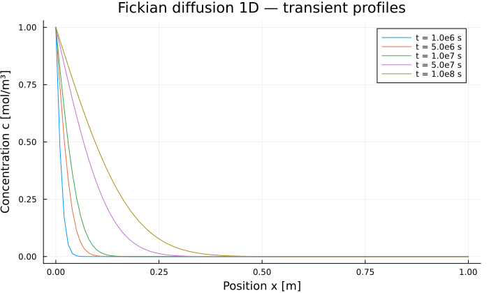

Comparison with the analytical solution

The numerical profile is compared with the semi-infinite erfc solution at the final time.

c_num = tsol[1, :, end]
c_ref = C_IN .* erfc.(xcoords ./ (2 * sqrt(model.D * t_end)))

err_L2 = sqrt(sum((c_num .- c_ref) .^ 2) / length(c_num))
err_Linf = maximum(abs.(c_num .- c_ref))

@printf("L2 error   : %.2e mol/m³\n", err_L2)
@printf("L∞ error   : %.2e mol/m³\n", err_Linf)
err_Linf < 0.01 * C_IN ? println("✓ err < 1 %") : println("✗ err > 1 %")

L2 error   : 3.37e-04 mol/m³
L∞ error   : 9.53e-04 mol/m³
✓ err < 1 %

Key points

• IC/BC consistency — the initial condition must satisfy the Dirichlet condition at node x=0 from t=0 (inival[1,1] = C_IN). Without it the adaptive controller sees Δu = C_IN regardless of Δt, and shrinks the time step until Δt_min.

• Implicit zero Neumann — VoronoiFVM applies zero flux by default on any boundary that bcondition! does not handle, so x = L needs no boundary_neumann! call.

• Δu_opt — set to 0.1 mol/m³, 10 % of C_IN: VoronoiFVM adapts Δt so that the largest concentration change per step stays under that threshold.