Bases
Basis types and their accessors. Theory: Bases and variance; usage: Bases.
TensND.Basis Type
Basis(v::AbstractMatrix{T}, ::Val{:cov})
Basis{dim, T<:Number}()
Basis(θ::T<:Number, ϕ::T<:Number, ψ::T<:Number)
Basis built from a square matrix v where columns correspond either to
primal vectors ie
eᵢ=v[:,i]ifvar=:covas by defaultdual vectors ie
eⁱ=v[:,i]ifvar=:cont.
Basis without any argument refers to the canonical basis (CanonicalBasis) in Rᵈⁱᵐ (by default dim=3 and T=Sym)
Basis can also be built from Euler angles (RotatedBasis) θ in 2D and (θ, ϕ, ψ) in 3D
The attributes of this object can be obtained by
vecbasis(ℬ, :cov): square matrix defining the primal basiseᵢ=e[:,i]vecbasis(ℬ, :cont): square matrix defining the dual basiseⁱ=E[:,i]metric(ℬ, :cov): square matrix defining the covariant components of the metric tensorgᵢⱼ=eᵢ⋅eⱼ=g[i,j]metric(ℬ, :cont): square matrix defining the contravariant components of the metric tensorgⁱʲ=eⁱ⋅eʲ=gⁱʲ[i,j]
Examples
julia> v = Sym[1 0 0; 0 1 0; 0 1 1] ; ℬ = Basis(v)
Basis{3, Sym}
# basis: 3×3 Tensor{2, 3, Sym, 9}:
 1  0  0
 0  1  0
 0  1  1
# dual basis: 3×3 Tensor{2, 3, Sym, 9}:
 1  0   0
 0  1  -1
 0  0   1
# covariant metric tensor: 3×3 SymmetricTensor{2, 3, Sym, 6}:
 1  0  0
 0  2  1
 0  1  1
# contravariant metric tensor: 3×3 SymmetricTensor{2, 3, Sym, 6}:
 1   0   0
 0   1  -1
 0  -1   2

julia> θ, ϕ, ψ = symbols("θ, ϕ, ψ", real = true) ; ℬʳ = Basis(θ, ϕ, ψ) ; display(vecbasis(ℬʳ, :cov))
3×3 Tensor{2, 3, Sym, 9}:
 -sin(ψ)⋅sin(ϕ) + cos(θ)⋅cos(ψ)⋅cos(ϕ)  -sin(ψ)⋅cos(θ)⋅cos(ϕ) - sin(ϕ)⋅cos(ψ)  sin(θ)⋅cos(ϕ)
  sin(ψ)⋅cos(ϕ) + sin(ϕ)⋅cos(θ)⋅cos(ψ)  -sin(ψ)⋅sin(ϕ)⋅cos(θ) + cos(ψ)⋅cos(ϕ)  sin(θ)⋅sin(ϕ)
                        -sin(θ)⋅cos(ψ)                          sin(θ)⋅sin(ψ)         cos(θ)
TensND.CanonicalBasis Type
CanonicalBasis{dim, T}Canonical basis of dimension dim (default: 3) and type T (default: Sym)
The attributes of this object can be obtained by
vecbasis(ℬ, :cov): square matrix defining the primal basiseᵢ=e[:,i]=δᵢⱼvecbasis(ℬ, :cont): square matrix defining the dual basiseⁱ=E[:,i]=δᵢⱼmetric(ℬ, :cov): square matrix defining the covariant components of the metric tensorgᵢⱼ=eᵢ⋅eⱼ=g[i,j]=δᵢⱼmetric(ℬ, :cont): square matrix defining the contravariant components of the metric tensorgⁱʲ=eⁱ⋅eʲ=gⁱʲ[i,j]=δᵢⱼ
Examples
julia> ℬ = CanonicalBasis()
CanonicalBasis{3, Sym}
# basis: 3×3 TensND.LazyIdentity{3, Sym}:
 1  0  0
 0  1  0
 0  0  1
# dual basis: 3×3 TensND.LazyIdentity{3, Sym}:
 1  0  0
 0  1  0
 0  0  1
# covariant metric tensor: 3×3 TensND.LazyIdentity{3, Sym}:
 1  0  0
 0  1  0
 0  0  1
# contravariant metric tensor: 3×3 TensND.LazyIdentity{3, Sym}:
 1  0  0
 0  1  0
 0  0  1

julia> ℬ₂ = CanonicalBasis{2, Float64}()
CanonicalBasis{2, Float64}
# basis: 2×2 TensND.LazyIdentity{2, Float64}:
 1.0  0.0
 0.0  1.0
# dual basis: 2×2 TensND.LazyIdentity{2, Float64}:
 1.0  0.0
 0.0  1.0
# covariant metric tensor: 2×2 TensND.LazyIdentity{2, Float64}:
 1.0  0.0
 0.0  1.0
# contravariant metric tensor: 2×2 TensND.LazyIdentity{2, Float64}:
 1.0  0.0
 0.0  1.0
TensND.RotatedBasis Type
RotatedBasis(θ::T<:Number, ϕ::T<:Number, ψ::T<:Number)
RotatedBasis(θ::T<:Number)
Orthonormal basis of dimension dim (default: 3) and type T (default: Sym) built from Euler angles θ in 2D and (θ, ϕ, ψ) in 3D
Examples
julia> θ, ϕ, ψ = symbols("θ, ϕ, ψ", real = true) ; ℬʳ = RotatedBasis(θ, ϕ, ψ) ; display(vecbasis(ℬʳ, :cov))
3×3 Tensor{2, 3, Sym, 9}:
 -sin(ψ)⋅sin(ϕ) + cos(θ)⋅cos(ψ)⋅cos(ϕ)  -sin(ψ)⋅cos(θ)⋅cos(ϕ) - sin(ϕ)⋅cos(ψ)  sin(θ)⋅cos(ϕ)
  sin(ψ)⋅cos(ϕ) + sin(ϕ)⋅cos(θ)⋅cos(ψ)  -sin(ψ)⋅sin(ϕ)⋅cos(θ) + cos(ψ)⋅cos(ϕ)  sin(θ)⋅sin(ϕ)
                        -sin(θ)⋅cos(ψ)                          sin(θ)⋅sin(ψ)         cos(θ)
TensND.OrthogonalBasis Type
OrthogonalBasis{dim,T}Orthogonal but not normalized basis: an orthonormal basis scaled by one factor χᵢ per direction.
Its metric is diagonal, gᵢⱼ = diag(χᵢ²), and its dual vectors are 𝐞ⁱ = 𝐞ᵢ/χᵢ², so variance still matters but only diagonally. This is exactly the situation of the natural basis of a curvilinear coordinate system, where the χᵢ are the Lamé coefficients — see Curvilinear differential calculus.
Built by Basis(ℬ, χᵢ) from an orthonormal basis and a tuple of scaling factors. Normalizing it returns the orthonormal basis it came from.
TensND.CylindricalBasis Function
CylindricalBasis(θ)Local orthonormal basis (𝐞ʳ, 𝐞ᶿ, 𝐞ᶻ) of the cylindrical system at azimuth θ, i.e. RotatedBasis(0, θ, 0).
Convenience constructor for a one-off local frame; for differential calculus use coorsys_cylindrical, which also carries the Lamé coefficients and the Christoffel symbols.
TensND.SphericalBasis Function
SphericalBasis(θ, ϕ)Local orthonormal basis (𝐞ᶿ, 𝐞ᵠ, 𝐞ʳ) of the spherical system at polar angle θ and azimuth ϕ, i.e. RotatedBasis(θ, ϕ, 0).
Note the ordering: the radial vector comes last, so that θ = ϕ = 0 returns the canonical basis in the canonical order. See Rotations and Euler angles.
Convenience constructor for a one-off local frame; for differential calculus use coorsys_spherical.
TensND.AllOrthogonalBasis Type
AllOrthogonalBasis{dim,T}Union of every basis whose metric is diagonal: the orthonormal ones (CanonicalBasis, RotatedBasis) and the merely orthogonal OrthogonalBasis.
Used to dispatch the component conversions that need no dense metric.
TensND.vecbasis Function
vecbasis(ℬ::AbstractBasis, var = :cov)Return the primal (if var = :cov) or dual (if var = :cont) basis
TensND.metric Function
metric(ℬ::AbstractBasis, var = :cov)Return the covariant (if var = :cov) or contravariant (if var = :cont) metric matrix
TensND.angles Function
angles(M::AbstractMatrix{T})Determine the Euler angles corresponding to the input matrix supposed to be a rotation matrix or at least a similarity
Examples
julia> θ, ϕ, ψ = symbols("θ, ϕ, ψ", real = true) ; ℬʳ = RotatedBasis(θ, ϕ, ψ) ; display(vecbasis(ℬʳ, :cov))
3×3 Tensor{2, 3, Sym, 9}:
 -sin(ψ)⋅sin(ϕ) + cos(θ)⋅cos(ψ)⋅cos(ϕ)  -sin(ψ)⋅cos(θ)⋅cos(ϕ) - sin(ϕ)⋅cos(ψ)  sin(θ)⋅cos(ϕ)
  sin(ψ)⋅cos(ϕ) + sin(ϕ)⋅cos(θ)⋅cos(ψ)  -sin(ψ)⋅sin(ϕ)⋅cos(θ) + cos(ψ)⋅cos(ϕ)  sin(θ)⋅sin(ϕ)
                        -sin(θ)⋅cos(ψ)                          sin(θ)⋅sin(ψ)         cos(θ)

julia> angles(ℬʳ)
(θ = θ, ϕ = ϕ, ψ = ψ)
TensND.isorthogonal Function
isorthogonal(ℬ::AbstractBasis)Check whether the basis ℬ is orthogonal
TensND.isorthonormal Function
isorthonormal(ℬ::AbstractBasis)Check whether the basis ℬ is orthonormal
TensND.get_dim Function
get_dim(t::AbstractTens) → Int
get_dim(ℬ::AbstractBasis) → Int
Dimension of the underlying space.
TensND.init_cartesian Function
init_cartesian(coords = symbols("x y z", real = true))Returns the coordinates, unit vectors and basis of the cartesian basis
Examples
julia> coords, vectors, ℬ = init_cartesian() ; x, y, z = coords ; 𝐞₁, 𝐞₂, 𝐞₃ = vectors ;TensND.init_polar Function
init_polar(coords = (symbols("r θ", real = true)); canonical = false)Returns the coordinates, base vectors and basis of the polar basis
Examples
julia> coords, vectors, ℬᵖ = init_polar() ; r, θ = coords ; 𝐞ʳ, 𝐞ᶿ = vectors ;TensND.init_cylindrical Function
init_cylindrical(coords = (symbols("r", positive = true), symbols("θ z", real = true)...); canonical = false)Returns the coordinates, base vectors and basis of the cylindrical basis
Examples
julia> coords, vectors, ℬᶜ = init_cylindrical() ; r, θ, z = coords ; 𝐞ʳ, 𝐞ᶿ, 𝐞ᶻ = vectors ;TensND.init_spherical Function
init_spherical(coords = (symbols("θ ϕ", real = true)..., symbols("r", positive = true)); canonical = false)Return the coordinates, base vectors and basis of the spherical basis. Take care that the order of the 3 vectors is 𝐞ᶿ, 𝐞ᵠ, 𝐞ʳ so that the basis coincides with the canonical one when the angles are null and in consistency the coordinates are ordered as θ, ϕ, r.
Examples
julia> coords, vectors, ℬˢ = init_spherical() ; θ, ϕ, r = coords ; 𝐞ᶿ, 𝐞ᵠ, 𝐞ʳ = vectors ;TensND.init_rotated Function
init_rotated(coords = symbols("θ ϕ ψ", real = true); canonical = false)Return the angles, base vectors and basis of the rotated basis. Note that here the coordinates are angles and do not represent a valid parametrization of ℝ³
Examples
julia> angles, vectors, ℬʳ = init_rotated() ; θ, ϕ, ψ = angles ; 𝐞ᶿ, 𝐞ᵠ, 𝐞ʳ = vectors ;