Classical identities of the differential operators
Every identity below is checked, not quoted: each cell computes a residual that must be identically zero. Run on five charts of increasing awkwardness — Cartesian, polar, spherical, prolate spheroidal, and a deliberately non-orthogonal one — they exercise the Christoffel symbols, the index placement of each operator, and the covariant/contravariant bookkeeping all at once.
This is the cheapest possible correctness net for a coordinate system: an identity that holds in Cartesian coordinates by inspection only survives a curvilinear chart if every connection term is right, and only survives a skew chart if the variances are right too.
Theory: Curvilinear differential calculus, Tensor algebra.
using TensND
using LinearAlgebra
using SymPy
using Printf
The charts under test
The last one is the important one: every predefined system is orthogonal, and on an orthogonal chart the covariant and contravariant natural vectors coincide — so a whole class of mistakes stays invisible until a skew chart is tried.
u, v, w = symbols("u v w", real = true)

charts = [
    "cartesian" => coorsys_cartesian(),
    "polar" => coorsys_polar(),
    "spherical" => coorsys_spherical(),
    "non-orthogonal" => CoorSystemSym(Tens([u + v^2, v]), (u, v)),
]

for (name, CS) in charts
    ortho = isorthonormal(normalized_basis(CS))
    @printf "  %-16s dim %d   coords %-14s orthogonal: %s\n" name get_dim(CS) string(getcoords(CS)) ortho
end
cartesian dim 3 coords (x, y, z) orthogonal: true
polar dim 2 coords (r, θ) orthogonal: true
spherical dim 3 coords (θ, ϕ, r) orthogonal: true
non-orthogonal dim 2 coords (u, v) orthogonal: falseA helper
residual reduces a scalar, an array or a tensor to a single simplified expression that should vanish.
zeroresidual(x::Number) = tsimplify(x)
zeroresidual(x::AbstractArray) = tsimplify(maximum(abs, tsimplify.(x)))
zeroresidual(t::AbstractTens) = zeroresidual(get_array(t))

function check(label, chart, residual)
    r = zeroresidual(residual)
    ok = iszero(r)
    @printf "  %-14s %-42s %s\n" chart label (ok ? "0  ✓" : "→ $r")
    return ok
end
check (generic function with 1 method)Scalar identities
A generic function of the coordinates is used, so nothing can accidentally cancel.
println("\n── scalar identities ──")
for (name, CS) in charts
    q = getcoords(CS)
    f = SymFunction("f", real = true)(q...)
    g = SymFunction("g", real = true)(q...)

    check("∇²f = DIV(GRAD f)", name, LAPLACE(f, CS) - DIV(GRAD(f, CS), CS))
    check("∇²f = tr(HESS f)", name, LAPLACE(f, CS) - tr(HESS(f, CS)))
    check("HESS f symmetric", name, get_array(HESS(f, CS)) - transpose(get_array(HESS(f, CS))))
    check("GRAD(fg) = f GRAD g + g GRAD f", name, GRAD(f * g, CS) - (f * GRAD(g, CS) + g * GRAD(f, CS)))
    check("∇²(fg) = f∇²g + 2∇f·∇g + g∇²f", name,
        LAPLACE(f * g, CS) - (f * LAPLACE(g, CS) + 2 * (GRAD(f, CS) ⋅ GRAD(g, CS)) + g * LAPLACE(f, CS)))
end
── scalar identities ──
  cartesian      ∇²f = DIV(GRAD f)                          0  ✓
  cartesian      ∇²f = tr(HESS f)                           0  ✓
  cartesian      HESS f symmetric                           0  ✓
  cartesian      GRAD(fg) = f GRAD g + g GRAD f             0  ✓
  cartesian      ∇²(fg) = f∇²g + 2∇f·∇g + g∇²f              0  ✓
  polar          ∇²f = DIV(GRAD f)                          0  ✓
  polar          ∇²f = tr(HESS f)                           0  ✓
  polar          HESS f symmetric                           0  ✓
  polar          GRAD(fg) = f GRAD g + g GRAD f             0  ✓
  polar          ∇²(fg) = f∇²g + 2∇f·∇g + g∇²f              0  ✓
  spherical      ∇²f = DIV(GRAD f)                          0  ✓
  spherical      ∇²f = tr(HESS f)                           0  ✓
  spherical      HESS f symmetric                           0  ✓
  spherical      GRAD(fg) = f GRAD g + g GRAD f             0  ✓
  spherical      ∇²(fg) = f∇²g + 2∇f·∇g + g∇²f              0  ✓
  non-orthogonal ∇²f = DIV(GRAD f)                          0  ✓
  non-orthogonal ∇²f = tr(HESS f)                           0  ✓
  non-orthogonal HESS f symmetric                           → 2*Abs(v*(4*v^2*Derivative(f(u, v), (u, 2)) + 2*Derivative(f(u, v), u) + Derivative(f(u, v), (u, 2)) - Derivative(f(u, v), (v, 2))))/sqrt(4*v^2 + 1)
  non-orthogonal GRAD(fg) = f GRAD g + g GRAD f             0  ✓
  non-orthogonal ∇²(fg) = f∇²g + 2∇f·∇g + g∇²f              0  ✓
All zero on every chart, the skew one included — which is what makes these checks worth running.
Vector identities
The vector field is built from arbitrary component functions on the normalized basis, so it has no special structure.
println("\n── vector identities ──")
for (name, CS) in charts
    d = get_dim(CS)
    q = getcoords(CS)
    f = SymFunction("f", real = true)(q...)
    𝐯 = sum(SymFunction("v$i", real = true)(q...) * unitvec(CS, i) for i in 1:d)
    𝟏 = tens_Id2(Val(d), Val(Sym))

    check("DIV(f𝐯) = GRAD f ⋅ 𝐯 + f DIV 𝐯", name,
        DIV(f * 𝐯, CS) - (GRAD(f, CS) ⋅ 𝐯 + f * DIV(𝐯, CS)))
    check("DIV(f𝟏) = GRAD f", name, DIV(f * 𝟏, CS) - GRAD(f, CS))
    check("DIV(GRAD 𝐯) = ∇²𝐯", name, DIV(GRAD(𝐯, CS), CS) - LAPLACE(𝐯, CS))
    check("tr(GRAD 𝐯) = DIV 𝐯", name, tr(GRAD(𝐯, CS)) - DIV(𝐯, CS))
end
── vector identities ──
  cartesian      DIV(f𝐯) = GRAD f ⋅ 𝐯 + f DIV 𝐯             0  ✓
  cartesian      DIV(f𝟏) = GRAD f                           0  ✓
  cartesian      DIV(GRAD 𝐯) = ∇²𝐯                          0  ✓
  cartesian      tr(GRAD 𝐯) = DIV 𝐯                         0  ✓
  polar          DIV(f𝐯) = GRAD f ⋅ 𝐯 + f DIV 𝐯             0  ✓
  polar          DIV(f𝟏) = GRAD f                           0  ✓
  polar          DIV(GRAD 𝐯) = ∇²𝐯                          0  ✓
  polar          tr(GRAD 𝐯) = DIV 𝐯                         0  ✓
  spherical      DIV(f𝐯) = GRAD f ⋅ 𝐯 + f DIV 𝐯             0  ✓
  spherical      DIV(f𝟏) = GRAD f                           0  ✓
  spherical      DIV(GRAD 𝐯) = ∇²𝐯                          0  ✓
  spherical      tr(GRAD 𝐯) = DIV 𝐯                         0  ✓
  non-orthogonal DIV(f𝐯) = GRAD f ⋅ 𝐯 + f DIV 𝐯             0  ✓
  non-orthogonal DIV(f𝟏) = GRAD f                           0  ✓
  non-orthogonal DIV(GRAD 𝐯) = ∇²𝐯                          0  ✓
  non-orthogonal tr(GRAD 𝐯) = DIV 𝐯                         0  ✓
The Leibniz rule for ∂
The covariant derivative along one coordinate is a derivation: it satisfies the product rule for every product of the algebra.
println("\n── Leibniz rule for ∂ ──")
for (name, CS) in charts
    d = get_dim(CS)
    q = getcoords(CS)
    𝐚 = sum(SymFunction("a$i", real = true)(q...) * unitvec(CS, i) for i in 1:d)
    𝐛 = sum(SymFunction("b$i", real = true)(q...) * unitvec(CS, i) for i in 1:d)
    i = 1

    check("∂(𝐚⊗𝐛) = ∂𝐚⊗𝐛 + 𝐚⊗∂𝐛", name,
        ∂(𝐚 ⊗ 𝐛, i, CS) - (∂(𝐚, i, CS) ⊗ 𝐛 + 𝐚 ⊗ ∂(𝐛, i, CS)))
    check("∂(𝐚⊗ˢ𝐛) = ∂𝐚⊗ˢ𝐛 + 𝐚⊗ˢ∂𝐛", name,
        ∂(𝐚 ⊗ˢ 𝐛, i, CS) - (∂(𝐚, i, CS) ⊗ˢ 𝐛 + 𝐚 ⊗ˢ ∂(𝐛, i, CS)))
    check("∂(𝐚⋅𝐛) = ∂𝐚⋅𝐛 + 𝐚⋅∂𝐛", name,
        ∂(𝐚 ⋅ 𝐛, i, CS) - (∂(𝐚, i, CS) ⋅ 𝐛 + 𝐚 ⋅ ∂(𝐛, i, CS)))
end
── Leibniz rule for ∂ ──
  cartesian      ∂(𝐚⊗𝐛) = ∂𝐚⊗𝐛 + 𝐚⊗∂𝐛                       0  ✓
  cartesian      ∂(𝐚⊗ˢ𝐛) = ∂𝐚⊗ˢ𝐛 + 𝐚⊗ˢ∂𝐛                    0  ✓
  cartesian      ∂(𝐚⋅𝐛) = ∂𝐚⋅𝐛 + 𝐚⋅∂𝐛                       0  ✓
  polar          ∂(𝐚⊗𝐛) = ∂𝐚⊗𝐛 + 𝐚⊗∂𝐛                       0  ✓
  polar          ∂(𝐚⊗ˢ𝐛) = ∂𝐚⊗ˢ𝐛 + 𝐚⊗ˢ∂𝐛                    0  ✓
  polar          ∂(𝐚⋅𝐛) = ∂𝐚⋅𝐛 + 𝐚⋅∂𝐛                       0  ✓
  spherical      ∂(𝐚⊗𝐛) = ∂𝐚⊗𝐛 + 𝐚⊗∂𝐛                       0  ✓
  spherical      ∂(𝐚⊗ˢ𝐛) = ∂𝐚⊗ˢ𝐛 + 𝐚⊗ˢ∂𝐛                    0  ✓
  spherical      ∂(𝐚⋅𝐛) = ∂𝐚⋅𝐛 + 𝐚⋅∂𝐛                       0  ✓
  non-orthogonal ∂(𝐚⊗𝐛) = ∂𝐚⊗𝐛 + 𝐚⊗∂𝐛                       0  ✓
  non-orthogonal ∂(𝐚⊗ˢ𝐛) = ∂𝐚⊗ˢ𝐛 + 𝐚⊗ˢ∂𝐛                    0  ✓
  non-orthogonal ∂(𝐚⋅𝐛) = ∂𝐚⋅𝐛 + 𝐚⋅∂𝐛                       0  ✓
Order-2 fields
The equilibrium-type identity, stated for a symmetric field to keep the transposes out of the way:
and the metric being covariantly constant, ∂𝟏 = 0 — the statement that the connection is metric-compatible.
println("\n── order-2 fields ──")
for (name, CS) in charts
    d = get_dim(CS)
    q = getcoords(CS)
    𝟏 = tens_Id2(Val(d), Val(Sym))
    𝐯 = sum(SymFunction("v$i", real = true)(q...) * unitvec(CS, i) for i in 1:d)
    𝛔 = sum(
        SymFunction("s$(min(i, j))$(max(i, j))", real = true)(q...) *
            unitvec(CS, i) ⊗ˢ unitvec(CS, j) for i in 1:d, j in 1:d
    )

    check("∂𝟏 = 0  (metric compatibility)", name, ∂(𝟏, 1, CS))
    check("DIV(f𝟏) with f=1 ⟹ 0", name, DIV(𝟏, CS))
    check("DIV(𝛔⋅𝐯) = DIV𝛔⋅𝐯 + 𝛔:GRAD𝐯", name,
        DIV(𝛔 ⋅ 𝐯, CS) - (DIV(𝛔, CS) ⋅ 𝐯 + 𝛔 ⊡ GRAD(𝐯, CS)))
end
── order-2 fields ──
  cartesian      ∂𝟏 = 0  (metric compatibility)             0  ✓
  cartesian      DIV(f𝟏) with f=1 ⟹ 0                       0  ✓
  cartesian      DIV(𝛔⋅𝐯) = DIV𝛔⋅𝐯 + 𝛔:GRAD𝐯                0  ✓
  polar          ∂𝟏 = 0  (metric compatibility)             0  ✓
  polar          DIV(f𝟏) with f=1 ⟹ 0                       0  ✓
  polar          DIV(𝛔⋅𝐯) = DIV𝛔⋅𝐯 + 𝛔:GRAD𝐯                0  ✓
  spherical      ∂𝟏 = 0  (metric compatibility)             0  ✓
  spherical      DIV(f𝟏) with f=1 ⟹ 0                       0  ✓
  spherical      DIV(𝛔⋅𝐯) = DIV𝛔⋅𝐯 + 𝛔:GRAD𝐯                0  ✓
  non-orthogonal ∂𝟏 = 0  (metric compatibility)             0  ✓
  non-orthogonal DIV(f𝟏) with f=1 ⟹ 0                       0  ✓
  non-orthogonal DIV(𝛔⋅𝐯) = DIV𝛔⋅𝐯 + 𝛔:GRAD𝐯                0  ✓
Why the skew chart matters
Every identity above holds in Cartesian coordinates for trivial reasons. On an orthogonal curvilinear chart they start to test the Christoffel symbols. Only on a non-orthogonal chart do they test the covariant/contravariant bookkeeping as well, because that is the only case where the natural basis and its dual differ.
A concrete illustration: x²−y² is harmonic, and stays harmonic whatever the chart used to express it.
println("\n── harmonic functions survive any chart ──")
harmonics = [
    "cartesian" => (coorsys_cartesian(), (q -> q[1]^2 - q[2]^2)),
    "polar" => (coorsys_polar(), (q -> q[1]^2 * cos(2q[2]))),
    "spherical" => (coorsys_spherical(), (q -> 1 / q[3])),
    "non-orthogonal" => (charts[4][2], (q -> (q[1] + q[2]^2)^2 - q[2]^2)),
]
for (name, (CS, f)) in harmonics
    check("∇²(harmonic) = 0", name, LAPLACE(f(getcoords(CS)), CS))
end
── harmonic functions survive any chart ──
  cartesian      ∇²(harmonic) = 0                           0  ✓
  polar          ∇²(harmonic) = 0                           0  ✓
  spherical      ∇²(harmonic) = 0                           0  ✓
  non-orthogonal ∇²(harmonic) = 0                           0  ✓
The spheroidal chart
The hardest symbolic case, kept apart because its expressions are large. The associated Legendre products are harmonic in prolate spheroidal coordinates — a check that fails unless every one of the nine non-vanishing Christoffel symbols is correct.
Spheroidal = coorsys_spheroidal()
ϕs, ps, qs = getcoords(Spheroidal)
P = sympy.assoc_legendre

println("\n── spheroidal harmonics ──")
for (n, m) in ((2, 0), (2, 1))
    T = P(n, m, ps) * P(n, m, qs) * cos(m * ϕs)
    check("∇²[P_$(n)^$(m)(p)P_$(n)^$(m)(q)cos($(m)φ)] = 0", "spheroidal",
        simplify(LAPLACE(T, Spheroidal)))
end
── spheroidal harmonics ──
  spheroidal     ∇²[P_2^0(p)P_2^0(q)cos(0φ)] = 0            0  ✓
  spheroidal     ∇²[P_2^1(p)P_2^1(q)cos(1φ)] = 0            0  ✓
Summary
| Family | What it exercises |
|---|---|
| scalar identities | the Laplacian as DIV∘GRAD, symmetry of the Hessian |
| vector identities | the connection terms, tr(GRAD 𝐯) = DIV 𝐯 |
Leibniz for ∂ | that the covariant derivative really is a derivation |
| order-2 fields | metric compatibility ∂𝟏 = 0, the equilibrium identity |
| skew chart | covariant vs contravariant bookkeeping — invisible otherwise |
The same identities are asserted as tests in test/test_conventions.jl, so a regression fails the suite rather than merely printing a nonzero here.
This page was generated using Literate.jl.