Surfaces: fundamental forms and curvature
A SubManifoldSym is a hypersurface embedded in
Surface indices run from
Theory: Submanifolds.
using TensND
using LinearAlgebra
using SymPy
Resolving
SymPy cannot know that real, or even positive, still leaves rules argument of SubManifoldSym is exactly the mechanism for this: a rewrite applied after each simplification.
R = symbols("R", positive = true)
θ = symbols("θ", positive = true)
ϕ = symbols("ϕ", real = true)
z = symbols("z", real = true)
The sphere
The classical umbilical surface: every direction curves identically. The rewrite |sinθ| => sinθ is passed straight to the constructor.
Sphere = SubManifoldSym(
    Tens(R * [sin(θ)cos(ϕ), sin(θ)sin(ϕ), cos(θ)]), (θ, ϕ), (), (R,);
    rules = Dict(abs(sin(θ)) => sin(θ)),
)
SubManifoldSym{3, TensND.TensCanonical{1, 3, Sym{PyCall.PyObject}, Tensors.Vec{3, Sym{PyCall.PyObject}}}, RotatedBasis{3, Sym{PyCall.PyObject}}, OrthogonalBasis{3, Sym{PyCall.PyObject}}, TensND.TensOrthogonal{2, 3, Sym{PyCall.PyObject}, Tensors.SymmetricTensor{2, 3, Sym{PyCall.PyObject}, 6}}, TensND.TensOrthogonal{2, 3, Sym{PyCall.PyObject}, Tensors.SymmetricTensor{2, 3, Sym{PyCall.PyObject}, 6}}}(TensND.ChartCore{3, Sym, TensND.TensCanonical{1, 3, Sym{PyCall.PyObject}, Tensors.Vec{3, Sym{PyCall.PyObject}}}, RotatedBasis{3, Sym{PyCall.PyObject}}, OrthogonalBasis{3, Sym{PyCall.PyObject}}}(Sym{PyCall.PyObject}[R*sin(θ)*cos(ϕ), R*sin(θ)*sin(ϕ), R*cos(θ)], (θ, ϕ), Sym{PyCall.PyObject}[cos(θ)*cos(ϕ) -sin(ϕ) sin(θ)*cos(ϕ); sin(ϕ)*cos(θ) cos(ϕ) sin(θ)*sin(ϕ); -sin(θ) 0 cos(θ)], Sym{PyCall.PyObject}[R*cos(θ)*cos(ϕ) -R*sin(θ)*sin(ϕ) sin(θ)*cos(ϕ); R*sin(ϕ)*cos(θ) R*sin(θ)*cos(ϕ) sin(θ)*sin(ϕ); -R*sin(θ) 0 cos(θ)], (Sym{PyCall.PyObject}[R, 0, 0], Sym{PyCall.PyObject}[0, R*sin(θ), 0], Sym{PyCall.PyObject}[0, 0, 1]), (R, R*sin(θ), 1), (Sym{PyCall.PyObject}[1/R, 0, 0], Sym{PyCall.PyObject}[0, 1/(R*sin(θ)), 0], Sym{PyCall.PyObject}[0, 0, 1]), (Sym{PyCall.PyObject}[1, 0, 0], Sym{PyCall.PyObject}[0, 1, 0], Sym{PyCall.PyObject}[0, 0, 1]), Sym[0 0 1/R; 0 -sin(θ)*cos(θ) 0;;; 0 cos(θ)/sin(θ) 0; cos(θ)/sin(θ) 0 1/R;;; -R 0 0; 0 -R*sin(θ)^2 0], (), (R,), Dict{Sym{PyCall.PyObject}, Sym{PyCall.PyObject}}(Abs(sin(θ)) => sin(θ)), Dict{Any, Any}(), Dict{Any, Any}()), Sym{PyCall.PyObject}[R^2 0 0; 0 R^2*sin(θ)^2 0; 0 0 0], Sym{PyCall.PyObject}[-R 0 0; 0 -R*sin(θ)^2 0; 0 0 0])The unit normal is the radial vector:
tsimplify.(components_canon(normal(Sphere)))First fundamental form — the familiar
𝐚 = submetric(Sphere)
get_array(𝐚)
Second fundamental form:
𝐛 = curvature(Sphere)
tsimplify.(get_array(𝐛))
For a sphere with the outward normal,
tsimplify.(get_array(𝐛) + get_array(𝐚) / R)Curvatures
The shape operator is the second form with one index raised,
function curvatures(SM)
    dim = length(get_array(submetric(SM))[1, :])
    tang = 1:(dim - 1)
    a = tsimplify.(get_array(submetric(SM))[tang, tang])
    b = tsimplify.(get_array(curvature(SM))[tang, tang])
    S = tsimplify.(inv(a) * b)
    return (K = tsimplify(det(S)), H = tsimplify(tr(S) / (dim - 1)), shape = tsimplify.(diag(S)))
end

cs = curvatures(Sphere)
println("sphere : K = ", cs.K, "   H = ", cs.H, "   principal curvatures = ", cs.shape)
sphere : K = R^(-2) H = -1/R principal curvatures = Sym{PyCall.PyObject}[-1/R, -1/R]The cylinder
One principal curvature vanishes, so
Cylinder = SubManifoldSym(Tens([R * cos(ϕ), R * sin(ϕ), z]), (ϕ, z), (), (R,))

tsimplify.(get_array(submetric(Cylinder))), tsimplify.(get_array(curvature(Cylinder)))
(Sym{PyCall.PyObject}[R^2 0 0; 0 1 0; 0 0 0], Sym{PyCall.PyObject}[-R 0 0; 0 0 0; 0 0 0])cc = curvatures(Cylinder)
println("cylinder : K = ", cc.K, " H = ", cc.H, " principal curvatures = ", cc.shape)cylinder : K = 0 H = -1/(2*R) principal curvatures = Sym{PyCall.PyObject}[-1/R, 0]The plane
The degenerate case: the normal is constant, so
x, y = symbols("x y", real = true)
Plane = SubManifoldSym(Tens([x, y, zero(x)]), (x, y))

tsimplify.(get_array(curvature(Plane)))cp = curvatures(Plane)
println("plane : K = ", cp.K, " H = ", cp.H)plane : K = 0 H = 0A paraboloid
A surface whose curvature actually varies with position.
Paraboloid = SubManifoldSym(Tens([x, y, (x^2 + y^2) / (2R)]), (x, y), (), (R,))
pb = curvatures(Paraboloid)
(K = R^2/(R^4 + 2*R^2*x^2 + 2*R^2*y^2 + x^4 + 2*x^2*y^2 + y^4), H = (2*R^2 + x^2 + y^2)/(2*(R^2 + x^2 + y^2)^(3/2)), shape = Sym{PyCall.PyObject}[(R^2 + y^2)/(R^2 + x^2 + y^2)^(3/2), (R^2 + x^2)/(R^2 + x^2 + y^2)^(3/2)])The closed forms are large, so they are more usefully read as values. At the apex
Note the sign: the
println("  s = √(x²+y²)      K·R²           H·R")
for s in (0.0, 0.5, 1.0, 2.0, 4.0)
    sub = Dict(x => Sym(s), y => Sym(0), R => Sym(1))
    Kv = Float64(simplify(pb.K.subs(sub)))
    Hv = Float64(simplify(pb.H.subs(sub)))
    println("     ", rpad(s, 12), rpad(round(Kv, digits = 8), 15), round(Hv, digits = 8))
end
s = √(x²+y²) K·R² H·R
0.0 1.0 1.0
0.5 0.64 0.80498447
1.0 0.25 0.53033009
2.0 0.04 0.26832816
4.0 0.00346021 0.12840121The apex values, symbolically:
(simplify(pb.K.subs(Dict(x => Sym(0), y => Sym(0)))), simplify(pb.H.subs(Dict(x => Sym(0), y => Sym(0)))))(R^(-2), 1/R)The Weingarten relation as a gradient
Because a SubManifoldSym is a coordinate system, the differential operators apply to fields defined on the surface. The identity tying the two geometries together is
G = GRAD(normal(Sphere), Sphere)Compare tensors, not stored arrays
The two sides are stored on different bases and variances, so subtracting their get_arrays gives a nonzero — and rather convincing — wrong answer. On a sphere of radius
tsimplify.(get_array(G)), tsimplify.(get_array(𝐛))(Sym{PyCall.PyObject}[1/R 0 0; 0 1/R 0; 0 0 0], Sym{PyCall.PyObject}[-R 0 0; 0 -R*sin(θ)^2 0; 0 0 0])Brought to a common basis and variance the difference is exactly zero, in every variance:
ℬnat = natural_basis(Sphere)
for var in ((:cov, :cov), (:cont, :cov), (:cov, :cont), (:cont, :cont))
    resid = tsimplify.(components(G, ℬnat, var) + components(𝐛, ℬnat, var))
    println("  variance ", var, " : all zero ? ", all(iszero, resid))
end
variance (:cov, :cov) : all zero ? true
variance (:cont, :cov) : all zero ? true
variance (:cov, :cont) : all zero ? true
variance (:cont, :cont) : all zero ? trueThis is the practical face of Bases and variance: a tensor is not its component array, and only components in the same basis may be compared.
Intrinsic connection coefficients
connection returns the connection coefficients Riemann, which named the wrong object.) For the sphere:
Γ = connection(Sphere)
println("Γ^θ_ϕϕ = ", tsimplify(Γ[2, 2, 1]))
println("Γ^ϕ_θϕ = ", tsimplify(Γ[1, 2, 2]), "     Γ^ϕ_ϕθ = ", tsimplify(Γ[2, 1, 2]))
Γ^θ_ϕϕ = -sin(2*θ)/2
Γ^ϕ_θϕ = 1/tan(θ) Γ^ϕ_ϕθ = 1/tan(θ)They are not tensor components: they change inhomogeneously under a change of chart and can be made to vanish at any single point, which no curvature can. The intrinsic curvature is the
Summary
| Surface | comment | ||
|---|---|---|---|
| plane | |||
| sphere, radius | umbilical | ||
| cylinder, radius | intrinsically flat | ||
| paraboloid | varies | varies |
This page was generated using Literate.jl.