Christoffel symbols
The connection coefficients are what distinguish a derivative in a curvilinear chart from a plain partial derivative. This tutorial computes them from their definition, checks that definition term by term, tabulates them for every predefined system, confirms that the symbolic and the automatic-differentiation routes agree, and builds a non-trivial custom chart.
Theory: Curvilinear differential calculus.
Storage convention
Christoffel returns an array indexed Γ[i,j,k]
using TensND
using LinearAlgebra
using SymPy
using Printf
Checking the definition term by term
Compute
Spherical = coorsys_spherical()
coords = getcoords(Spherical)
Γ = Christoffel(Spherical)
d = 3

residuals = [
    tsimplify(
        ∂(natvec(Spherical, j, :cov), coords[i], Spherical) ⋅ natvec(Spherical, k, :cont)
            - Γ[i, j, k],
    )
        for i in 1:d, j in 1:d, k in 1:d
]
println("all Γ recovered from the definition ? ", all(iszero, residuals))
all Γ recovered from the definition ? trueSymmetry in the lower pair,
tsimplify(maximum(abs.(Γ - permutedims(Γ, (2, 1, 3)))))Every predefined system
Only the non-vanishing symbols are listed.
function christoffel_table(name, CS)
    c = getcoords(CS)
    G = Christoffel(CS)
    dim = length(c)
    println("── ", name, "   coords = ", c, "   Lamé = ", Lame(CS))
    any_nz = false
    for i in 1:dim, j in 1:dim, k in 1:dim
        v = tsimplify(G[i, j, k])
        if !iszero(v)
            @printf "     Γ^%s_%s%s = %s\n" string(c[k]) string(c[i]) string(c[j]) string(v)
            any_nz = true
        end
    end
    any_nz || println("     (all vanish — this is a Cartesian chart)")
    return println()
end

christoffel_table("cartesian", coorsys_cartesian())
christoffel_table("polar", coorsys_polar())
christoffel_table("cylindrical", coorsys_cylindrical())
christoffel_table("spherical", coorsys_spherical())
── cartesian coords = (x, y, z) Lamé = (1, 1, 1)
(all vanish — this is a Cartesian chart)
── polar coords = (r, θ) Lamé = (1, r)
Γ^θ_rθ = 1/r
Γ^θ_θr = 1/r
Γ^r_θθ = -r
── cylindrical coords = (r, θ, z) Lamé = (1, r, 1)
Γ^θ_rθ = 1/r
Γ^θ_θr = 1/r
Γ^r_θθ = -r
── spherical coords = (θ, ϕ, r) Lamé = (r, r*sin(θ), 1)
Γ^r_θθ = -r
Γ^ϕ_θϕ = 1/tan(θ)
Γ^θ_θr = 1/r
Γ^ϕ_ϕθ = 1/tan(θ)
Γ^θ_ϕϕ = -sin(2*θ)/2
Γ^r_ϕϕ = -r*sin(θ)^2
Γ^ϕ_ϕr = 1/r
Γ^θ_rθ = 1/r
Γ^ϕ_rϕ = 1/rThe Cartesian chart is precisely the one whose connection vanishes; everything else pays a
Why they matter
The divergence of the radial unit vector is
θ, ϕ, r = getcoords(Spherical)
𝐞ᶿ, 𝐞ᵠ, 𝐞ʳ = unitvec(Spherical)
@set_coorsys Spherical

get_array(𝐞ʳ), tsimplify(DIV(𝐞ʳ))
(Sym{PyCall.PyObject}[0, 0, 1], 2/r)Symbolic and numerical routes agree
CoorSystemNum evaluates the same geometry pointwise with ForwardDiff instead of SymPy. The Christoffel closure uses the same
CSnum = coorsys_spherical_num()
x₀ = [0.7, 1.1, 2.3]                       # (θ, ϕ, r)

Γnum = Christoffel(CSnum, x₀)
Γsym = [Float64(tsimplify(Γ[i, j, k]).subs(Dict(θ => x₀[1], ϕ => x₀[2], r => x₀[3]))) for i in 1:3, j in 1:3, k in 1:3]

println("‖Γ_num − Γ_sym‖ at (θ,ϕ,r) = ", x₀, " : ", norm(Γnum - Γsym))
‖Γ_num − Γ_sym‖ at (θ,ϕ,r) = [0.7, 1.1, 2.3] : 3.510833468576701e-16The same for the Lamé coefficients
(Lame(CSnum, x₀), (x₀[3], x₀[3] * sin(x₀[1]), 1.0))([2.3, 1.4817006806466892, 1.0], (2.3, 1.4817006806466892, 1.0))A custom chart: prolate spheroidal coordinates
Non-trivial charts produce metric expressions SymPy will not reduce on its own. CoorSystemSym therefore accepts auxiliary variables and rewrite rules — tmp_coords standing for compound expressions, tmp_var substituting them in, and to_coords eliminating them again before differentiation.
Prolate spheroidal coordinates
Spheroidal = coorsys_spheroidal()
getcoords(Spheroidal)
(ϕ, p, q)components_canon(getOM(Spheroidal))The Lamé coefficients, which without the simplification machinery come out as unreadable nested radicals:
Lame(Spheroidal)(c*sqrt(1 - p^2)*sqrt(q^2 - 1), c*sqrt(-p^2 + q^2)/sqrt(1 - p^2), c*sqrt(-p^2 + q^2)/sqrt(q^2 - 1))A harmonic check: the first Cartesian coordinate squared has Laplacian 2, whatever the chart used to compute it.
simplify(LAPLACE(getOM(Spheroidal)[1]^2, Spheroidal))Spheroidal harmonics
Associated Legendre products
ϕs, ps, qs = getcoords(Spheroidal)
P = sympy.assoc_legendre

for (n, m) in ((2, 0), (2, 1), (3, 2))
    T = P(n, m, ps) * P(n, m, qs) * cos(m * ϕs)
    lap = simplify(LAPLACE(T, Spheroidal))
    @printf "  ∇²[P_%d^%d(p) P_%d^%d(q) cos(%dφ)] = %s\n" n m n m m string(lap)
end
∇²[P_2^0(p) P_2^0(q) cos(0φ)] = 0
∇²[P_2^1(p) P_2^1(q) cos(1φ)] = 0
∇²[P_3^2(p) P_3^2(q) cos(2φ)] = 0Building a chart from an OM function alone
The numerical route needs no symbolic setup at all: hand CoorSystemNum a differentiable position map and it derives the Lamé coefficients, the rotation to the normalized frame and the Christoffel symbols by automatic differentiation.
Elliptic coordinates in the plane,
a_ell = 2.0
OM_elliptic = x -> [a_ell * cosh(x[1]) * cos(x[2]), a_ell * sinh(x[1]) * sin(x[2])]
CS_ell = CoorSystemNum(OM_elliptic, 2)

x_ell = [1.0, 0.8]
χ_ell = Lame(CS_ell, x_ell)
χ_exact = a_ell * sqrt(sinh(x_ell[1])^2 + sin(x_ell[2])^2)
println("Lamé  : ", round.(χ_ell, digits = 10), "   exact (both equal) : ", round(χ_exact, digits = 10))
Lamé : [2.7536866973, 2.7536866973] exact (both equal) : 2.7536866973lap_harm = LAPLACE(x -> cosh(x[1]) * cos(x[2]), CS_ell)(x_ell)
@printf "∇²(cosh μ cos ν) = %.3e (should vanish)\n" lap_harm∇²(cosh μ cos ν) = 1.388e-17 (should vanish)This page was generated using Literate.jl.