Differential operators, numerically
The same five operators as in Differential operators, symbolically, evaluated pointwise by automatic differentiation instead of SymPy. No symbolic setup, constant cost per point, and ForwardDiff.Dual numbers flow through — so a field computed this way can itself be differentiated with respect to a parameter.
Theory: Curvilinear differential calculus.
A CoorSystemNum stores its geometry as three closures — the Lamé coefficients, the rotation to the normalized frame, and the Christoffel symbols — all evaluated at the point of interest. A field is an ordinary Julia function of the coordinate vector, and an operator returns a function, which is then called at a point.
using TensND
using LinearAlgebra
using Printf
using ForwardDiff
Polar: the Laplacian of
The exact result is
CS_polar = coorsys_polar_num()
r₀, θ₀ = 2.5, 0.7

println("  n  m       numerical        exact")
for (n, m) in [(2, 1), (3, 1), (3, 3), (2, 2)]
    f = x -> x[1]^n * sin(m * x[2])
    num = LAPLACE(f, CS_polar)([r₀, θ₀])
    exact = (n^2 - m^2) * r₀^(n - 2) * sin(m * θ₀)
    @printf "  %d  %d   %+.10f   %+.10f\n" n m num exact
end
n m numerical exact
2 1 +1.9326530617 +1.9326530617
3 1 +12.8843537448 +12.8843537448
3 3 -0.0000000000 +0.0000000000
2 2 -0.0000000000 +0.0000000000Spherical: gradients and Laplacians of
Coordinates are ordered
CS_sph = coorsys_spherical_num()
x₀ = [π / 4, π / 3, 3.0]

println("   n     ∇[e_r]         exact          ∇²             exact")
for n in [1, 2, 3, -1]
    f = x -> x[3]^n
    g = GRAD(f, CS_sph)(x₀)
    lap = LAPLACE(f, CS_sph)(x₀)
    @printf "  %2d  %+.10f  %+.10f  %+.10f  %+.10f\n" n g[3] n * x₀[3]^(n - 1) lap n * (n + 1) * x₀[3]^(n - 2)
end
n ∇[e_r] exact ∇² exact
1 +1.0000000000 +1.0000000000 +0.6666666667 +0.6666666667
2 +6.0000000000 +6.0000000000 +6.0000000000 +6.0000000000
3 +27.0000000000 +27.0000000000 +36.0000000000 +36.0000000000
-1 -0.1111111111 -0.1111111111 +0.0000000000 +0.0000000000A field with angular dependence,
f_ang = x -> x[3]^2 * sin(x[1]) * cos(x[2])
g_num = GRAD(f_ang, CS_sph)(x₀)
g_exact = [
    x₀[3] * cos(x₀[1]) * cos(x₀[2]),      # e_θ
    -x₀[3] * sin(x₀[2]),                    # e_φ
    2x₀[3] * sin(x₀[1]) * cos(x₀[2]),     # e_r
]
(round.(g_num, digits = 10), round.(g_exact, digits = 10))
([1.0606601718, -2.5980762114, 2.1213203436], [1.0606601718, -2.5980762114, 2.1213203436])The Lamé problem: a hollow sphere under internal pressure
Inner radius
We take the displacement field as given and let the operators produce the strain, the stress and the equilibrium residual.
a, b = 1.0, 3.0
p_i = 1.0
κ, μ = 2.0, 1.0
λ = κ - 2μ / 3

A = p_i * a^3 / (3κ * (b^3 - a^3))
B = p_i * a^3 * b^3 / (4μ * (b^3 - a^3))

u_func = x -> [0.0, 0.0, A * x[3] + B / x[3]^2]          # (θ, φ, r) components
ε_func = x -> SYMGRAD(u_func, CS_sph)(x)
function σ_func(x)
    ε = ε_func(x)
    trε = sum(ε[i, i] for i in 1:3)
    return [λ * trε * (i == j) + 2μ * ε[i, j] for i in 1:3, j in 1:3]
end
σ_func (generic function with 1 method)SYMGRAD of a displacement is the linearized strain directly; DIV of the stress is the equilibrium operator, which must vanish everywhere.
θc, ϕc = π / 3, π / 4
println("   r      ε_rr        exact       ε_θθ        exact       σ_rr        exact      |div σ|")
for rv in [1.1, 1.5, 2.0, 2.5, 2.9]
    x = [θc, ϕc, rv]
    ε, σ = ε_func(x), σ_func(x)
    divσ = norm(DIV(σ_func, CS_sph)(x))
    @printf "  %.1f  %+.7f  %+.7f  %+.7f  %+.7f  %+.7f  %+.7f  %.1e\n" rv ε[3, 3] (A - 2B / rv^3) ε[1, 1] (A + B / rv^3) σ[3, 3] (3κ * A - 4μ * B / rv^3) divσ
end
r ε_rr exact ε_θθ exact σ_rr exact |div σ|
1.1 -0.3836955 -0.3836955 +0.2014631 +0.2014631 -0.7417500 -0.7417500 4.5e-16
1.5 -0.1474359 -0.1474359 +0.0833333 +0.0833333 -0.2692308 -0.2692308 2.3e-17
2.0 -0.0584936 -0.0584936 +0.0388622 +0.0388622 -0.0913462 -0.0913462 2.3e-18
2.5 -0.0268205 -0.0268205 +0.0230256 +0.0230256 -0.0280000 -0.0280000 4.2e-17
2.9 -0.0148793 -0.0148793 +0.0170550 +0.0170550 -0.0041176 -0.0041176 1.4e-17Equilibrium holds to machine precision at every radius, which is a genuine check: it exercises the full order-2 divergence, connection terms included.
The boundary conditions,
(σ_func([θc, ϕc, a])[3, 3], σ_func([θc, ϕc, b])[3, 3])(-1.0000000000000002, -6.938893903907228e-18)Differentiating through the operators
The operators are built on ForwardDiff, and they compose with it: an operator result can itself be differentiated with respect to the evaluation point. The Laplacian of
∇lap = ForwardDiff.gradient(x -> LAPLACE(y -> y[3]^3, CS_sph)(x), x₀)
round.(∇lap, digits = 10)
3-element Vector{Float64}:
-0.0
0.0
12.0The same for a tensor-valued field — the radial strain of
∇ε = ForwardDiff.gradient(x -> SYMGRAD(y -> [0.0, 0.0, y[3]^2], CS_sph)(x)[3, 3], x₀)
round.(∇ε, digits = 10)
3-element Vector{Float64}:
0.0
0.0
2.0... and with respect to a parameter carried by the field
The other direction works too: the internal buffers promote the element type of the geometry with that of the field, so a Dual-valued field on a Float64 coordinate system is handled correctly.
The Laplacian of
ForwardDiff.derivative(α -> LAPLACE(x -> α * x[3]^2, CS_sph)(x₀), 3.0)6.0For a tensor-valued field: the radial strain of
ForwardDiff.derivative(α -> SYMGRAD(x -> [zero(α), zero(α), α * x[3]], CS_sph)(x₀)[3, 3], 2.0)1.0And through a divergence —
dαdiv = ForwardDiff.derivative(α -> DIV(x -> α * [0.0 0 0; 0 0 0; 0 0 1], CS_sph)(x₀)[3], 2.0)
(dαdiv, 2 / x₀[3])
(0.6666666666666666, 0.6666666666666666)Sensitivity of the Lamé solution
Putting the two together: the derivative of the hoop strain at mid-thickness with respect to the applied pressure, taken straight through a numerical SYMGRAD. The solution is linear in
function εθθ_of_p(pv)
    Av = pv * a^3 / (3κ * (b^3 - a^3))
    Bv = pv * a^3 * b^3 / (4μ * (b^3 - a^3))
    u = x -> [zero(pv), zero(pv), Av * x[3] + Bv / x[3]^2]
    return SYMGRAD(u, CS_sph)([θc, ϕc, 2.0])[1, 1]
end

dε_ad = ForwardDiff.derivative(εθθ_of_p, p_i)
@printf "dε_θθ/dp : AD = %+.12f   exact = %+.12f\n" dε_ad (εθθ_of_p(p_i) / p_i)
dε_θθ/dp : AD = +0.038862179487 exact = +0.038862179487A custom system from an OM function
The generic constructor takes any differentiable position map. Elliptic coordinates,
a_ell = 2.0
CS_ell = CoorSystemNum(x -> [a_ell * cosh(x[1]) * cos(x[2]), a_ell * sinh(x[1]) * sin(x[2])], 2)
x_ell = [1.0, 0.8]

(Lame(CS_ell, x_ell), a_ell * sqrt(sinh(x_ell[1])^2 + sin(x_ell[2])^2))
([2.75368669727873, 2.75368669727873], 2.75368669727873)Two harmonic functions of this chart:
for (name, f) in ("μ" => (x -> x[1]), "cosh μ cos ν" => (x -> cosh(x[1]) * cos(x[2])))
    @printf "  ∇²(%-12s) = %+.3e\n" name LAPLACE(f, CS_ell)(x_ell)
end
∇²(μ ) = +0.000e+00
∇²(cosh μ cos ν) = +1.388e-17Symbolic or numerical?
| symbolic | numerical | |
|---|---|---|
| result | a formula, valid everywhere | a number, at one point |
| cost | grows with expression size | constant per point |
| needs | a symbolic | any differentiable OM(x) |
| best for | deriving closed forms | field evaluation, sweeps, gradients |
The two agree wherever both apply — checked in Christoffel symbols — so the choice is one of purpose, not of accuracy.
This page was generated using Literate.jl.