Submanifolds
A hypersurface embedded in TensND represents both with SubManifoldSym (src/submanifold.jl), which is a CoorSystemSym with one coordinate fewer than the ambient dimension and a unit normal completing the frame.
Tangent frame and normal
Let
and the frame is closed by the unit normal
The two fundamental forms
— the first fundamental form, the metric induced by the embedding. It measures lengths and angles within the surface and knows nothing of the ambient space. submetric.— the second fundamental form, the normal component of the variation of the tangent frame. It measures how the surface bends in the ambient space. curvature.
The second equality follows from
Both are stored as
Gauss and Weingarten
Decomposing
SubManifoldSym stores exactly this: the connection array
connection, formerly Riemann
connection returns the purely tangential block Riemann, is now connection. The old name still works and forwards, with a deprecation warning.
For a sphere of radius
which are indeed the sphere's connection coefficients. The name is The intrinsic curvature is recovered from
Curvatures
With the shape operator
| Quantity | Definition | Sphere of radius |
|---|---|---|
| principal curvatures | eigenvalues | |
| mean curvature | ||
| Gaussian curvature |
Gauss's Theorema Egregium is that
Worked closed forms
For a sphere of radius
The proportionality
| Surface | Comment | ||
|---|---|---|---|
| plane | |||
| sphere, radius | umbilical | ||
| cylinder, radius | intrinsically flat |
Differential operators on the surface
Because SubManifoldSym is an AbstractCoorSystem, the operators GRAD, DIV, LAPLACE apply to fields defined on the surface, with the intrinsic connection. The relation that ties the two geometries together is the Weingarten equation read as a gradient:
It is the cheapest check that an implementation's normal orientation and curvature sign agree, and it is pinned by a test (Testing and conventions).
Compare tensors, not stored arrays
This is an identity between tensors, and the two sides are not stored the same way: get_arrays therefore gives a nonzero, and rather convincing, wrong answer — on a sphere of radius
Bring both to a common basis and variance first — components(t, ℬ, var) or change_tens — after which the difference is exactly zero in every variance. This is the practical face of Bases and variance: a tensor is not its component array, and only components in the same basis may be compared.
Declare the parameter ranges, or fight Abs
Declaring real leaves SymPy unable to reduce rules of SubManifoldSym — or restrict the symbol's assumptions — so that the sign is resolved. This is the same simplification machinery described on Curvilinear differential calculus.