Coordinate systems (symbolic)
Differential operators on tensor fields, with exact symbolic derivatives. The mathematics — natural basis, Lamé coefficients, Christoffel symbols, the index placement of each operator — is on Curvilinear differential calculus.
Predefined systems
| Constructor | Coordinates | Lamé |
|---|---|---|
coorsys_cartesian | ||
coorsys_polar | ||
coorsys_cylindrical | ||
coorsys_spherical | ||
coorsys_spheroidal | prolate spheroidal |
Spherical coordinates are ordered (\theta,\varphi,r)
Not
The operators
using TensND, SymPy

Polar = coorsys_polar()
r, θ = getcoords(Polar)
𝐞ʳ, 𝐞ᶿ = unitvec(Polar)
@set_coorsys Polar

LAPLACE(SymFunction("f", real = true)(r, θ))
@set_coorsys installs a default system so the operators take one argument; without it, pass the system explicitly, LAPLACE(f, Polar).
| Call | Does |
|---|---|
@set_coorsysCS / set_coorsys!(CS) | make CS the default |
default_coorsys() | the current default (throws if none) |
unset_coorsys!() | forget it |
∂ is deliberately not affected by the default
∂(t, x) always means the plain derivative of t with respect to the symbol x; for the covariant derivative pass the chart explicitly, ∂(t, x, CS).
Earlier versions had @set_coorsys define methods in the TensND module, including one for ∂(t, x). That method was more specific than the plain-derivative fallback, so the same call silently changed meaning — and since both CoorSystemSym and SubManifoldSym differentiate a position vector while being built, constructing any new chart after a @set_coorsys failed. The default is now simply stored, and the single-argument operator methods are defined once.
| Operator | Order | Meaning |
|---|---|---|
GRAD | gradient, derivative index appended on the right | |
SYMGRAD | symmetrized gradient; for a displacement, the strain | |
DIV | divergence, contracting the last index | |
LAPLACE | ||
HESS |
n = symbols("n", integer = true)
simplify(LAPLACE(r^n * cos(n * θ)))
Accessors
| Function | Returns |
|---|---|
getcoords | the coordinate symbols |
getOM | the position vector |
unitvec | vectors of the normalized basis |
natvec | vectors of the natural basis (:cov or :cont) |
normalized_basis, natural_basis | the two bases |
Lame | the |
Christoffel | the array |
∂ | the covariant derivative along one coordinate |
using TensND, SymPy
Spherical = coorsys_spherical()
Lame(Spherical)
(r, r*sin(θ), 1)Christoffel(Spherical)[1, 1, 3] # Γʳ_θθ = −rCustom systems
CoorSystemSym(OM, coords, tmp_coords = (), params = ();
              rules = Dict(), tmp_var = Dict(), to_coords = Dict())
The position vector and the coordinate symbols suffice; the natural basis, Lamé coefficients and Christoffel symbols are derived. A variant takes the normalized basis and the
using TensND, SymPy

x, y = symbols("x y", real = true)
a = symbols("a", positive = true)
Parabolic = CoorSystemSym(Tens([(x^2 - y^2) / 2, x * y]), (x, y))
Lame(Parabolic)
(sqrt(x^2 + y^2), sqrt(x^2 + y^2))Taming symbolic expressions
Non-trivial charts produce metric expressions SymPy will not reduce unaided, and the Christoffel symbols become unusable nested radicals. Four optional arguments control this:
| Argument | Role |
|---|---|
tmp_coords | auxiliary symbols standing for compound expressions |
params | constants appearing in |
tmp_var | substitutions replacing expressions by those symbols |
to_coords | how to eliminate them again before differentiating |
rules | rewrite rules applied after each simplification |
The prolate spheroidal system is the standard illustration, and coorsys_spheroidal is built exactly this way:
Spheroidal = coorsys_spheroidal()
Lame(Spheroidal)
(c*sqrt(1 - p^2)*sqrt(q^2 - 1), c*sqrt(-p^2 + q^2)/sqrt(1 - p^2), c*sqrt(-p^2 + q^2)/sqrt(q^2 - 1))simplify(LAPLACE(getOM(Spheroidal)[1]^2, Spheroidal))rules is also what resolves sign ambiguities such as
Symbolic or numerical?
For pointwise evaluation, sweeps and gradients, use CoorSystemNum instead — same operator names, derivatives by automatic differentiation. See Numerical coordinate systems.