Coordinate systems (numerical)
The same five operators as in Coordinate systems, with derivatives taken by automatic differentiation instead of SymPy. No symbolic setup, constant cost per point, and results are numbers rather than formulas.
The key difference: operators return functions
A CoorSystemNum operator takes a field — an ordinary Julia function of the coordinate vector — and returns a function, which is then called at a point:
using TensND

CS = coorsys_spherical_num()
x₀ = [π / 4, π / 3, 3.0]          # (θ, φ, r)

LAPLACE(x -> x[3]^3, CS)(x₀) # ∇²(r³) = 12 r36.012 * x₀[3]36.0Predefined systems
| Constructor | Coordinates |
|---|---|
coorsys_cartesian_num | |
coorsys_polar_num | |
coorsys_cylindrical_num | |
coorsys_spherical_num |
The coordinate ordering matches the symbolic systems exactly, spherical included.
A custom system needs only a position map
CoorSystemNum(OM_func, dim)
CoorSystemNum(OM_func, dim, T)
OM_func maps a coordinate vector to the position vector and must be differentiable — nothing else is required. The Lamé coefficients, the rotation to the normalized frame and the Christoffel symbols are all derived by ForwardDiff.
a = 2.0
CS_ell = CoorSystemNum(x -> [a * cosh(x[1]) * cos(x[2]), a * sinh(x[1]) * sin(x[2])], 2)
x_ell = [1.0, 0.8]

Lame(CS_ell, x_ell), a * sqrt(sinh(x_ell[1])^2 + sin(x_ell[2])^2)
([2.75368669727873, 2.75368669727873], 2.75368669727873)LAPLACE(x -> cosh(x[1]) * cos(x[2]), CS_ell)(x_ell) # harmonic ⟹ 01.387778780781445e-17Pointwise accessors
Every accessor takes the point as an extra argument, because the geometry is stored as closures rather than expressions:
| Symbolic | Numerical |
|---|---|
Lame(CS) | Lame(CS, x₀) |
Christoffel(CS) | Christoffel(CS, x₀) |
normalized_basis(CS) | normalized_basis(CS, x₀) |
natural_basis(CS) | natural_basis(CS, x₀) |
unitvec(CS, i) | unitvec(CS, x₀, i) |
natvec(CS, i, var) | natvec(CS, x₀, i, var) |
The Christoffel array uses the same convention as the symbolic route,
round.(Christoffel(coorsys_spherical_num(), [0.7, 1.1, 2.3])[1, 1, 3], digits = 10)-2.3Composing with ForwardDiff
The operators are built on ForwardDiff and compose with it in both directions — with respect to the evaluation point, and with respect to a parameter carried by the field:
using TensND, ForwardDiff

CS = coorsys_spherical_num()
x₀ = [0.7, 1.1, 2.3]

ForwardDiff.gradient(x -> LAPLACE(y -> y[3]^3, CS)(x), x₀)   # ∇(12r)
3-element Vector{Float64}:
-1.7763568394002505e-15
0.0
12.0ForwardDiff.derivative(α -> LAPLACE(x -> α * x[3]^2, CS)(x₀), 3.0) # ∇²(αr²) = 6α6.0This makes a sensitivity analysis of a field problem a one-liner: wrap the computation in a function of the parameter and differentiate.
Choosing between the two routes
CoorSystemSym | CoorSystemNum | |
|---|---|---|
| derivatives | exact, symbolic | machine precision, AD |
| result | a formula, valid everywhere | a number, at one point |
| cost | grows with expression size | constant per point |
| needs | a symbolic | any differentiable OM(x) |
| best for | deriving closed forms | field evaluation, sweeps, gradients |
The two agree wherever both apply, which is checked in Christoffel symbols.