Submanifolds
Hypersurfaces embedded in
Construction
SubManifoldSym(OM, coords, tmp_coords = (), params = ();
               rules = Dict(), tmp_var = Dict(), to_coords = Dict())
coords holds one coordinate fewer than the ambient dimension: a surface in
using TensND, SymPy

R = symbols("R", positive = true)
θ = symbols("θ", positive = true)
ϕ = symbols("ϕ", real = true)

Sphere = SubManifoldSym(
    Tens(R * [sin(θ)cos(ϕ), sin(θ)sin(ϕ), cos(θ)]), (θ, ϕ), (), (R,);
    rules = Dict(abs(sin(θ)) => sin(θ)),
)
tsimplify.(components_canon(normal(Sphere)))
Use rules to resolve sign ambiguities
SymPy cannot know that rules argument rewrites it away, as above. The same machinery is described under Coordinate systems.
The four accessors
| Function | Returns |
|---|---|
normal | the unit normal |
submetric | the first fundamental form |
curvature | the second fundamental form |
connection | the intrinsic connection coefficients |
get_array(submetric(Sphere))tsimplify.(get_array(curvature(Sphere)))Both are returned as
For a sphere with the outward normal,
tsimplify.(get_array(curvature(Sphere)) + get_array(submetric(Sphere)) / R)The orientation decides the sign
The normal is the generalized cross product of the tangent vectors in the order given, so swapping two coordinates reverses it — and with it the sign of curvature and of the mean curvature. State the orientation whenever a curvature is reported. The Gaussian curvature, being a determinant, is unaffected.
connection — renamed from Riemann
connection returns the connection coefficients (Christoffel symbols) of the induced metric, never a Riemann curvature tensor. The old name Riemann named the wrong object; it still works and forwards, with a deprecation warning. For the sphere it gives submetric and curvature instead.
Curvatures
The shape operator is the second form with one index raised,
using LinearAlgebra
a2 = tsimplify.(get_array(submetric(Sphere))[1:2, 1:2])
b2 = tsimplify.(get_array(curvature(Sphere))[1:2, 1:2])
S = tsimplify.(inv(a2) * b2)
(tsimplify(det(S)), tsimplify(tr(S) / 2))
(R^(-2), -1/R)| Surface | ||
|---|---|---|
| plane | ||
| sphere, radius | ||
| cylinder, radius |
Differential operators on the surface
A SubManifoldSym is an AbstractCoorSystem, so GRAD, DIV and LAPLACE apply to fields defined on it, with the intrinsic connection. The identity linking the two geometries is the Weingarten relation read as a gradient,
Compare tensors, not stored arrays
The two sides are stored on different bases and variances, so subtracting their get_arrays gives a nonzero — and plausible-looking — wrong answer. Bring both to a common basis and variance first:
components(GRAD(normal(SM), SM), natural_basis(SM), (:cov, :cov)) +
components(curvature(SM),       natural_basis(SM), (:cov, :cov))
which is exactly zero. This is the practical face of Bases and variance.
A worked version of all of the above, on the sphere, cylinder, plane and paraboloid, is in Surfaces: fundamental forms and curvature.