Coordinate systems (symbolic)
Symbolic differential calculus on a curvilinear chart. Theory: Curvilinear differential calculus; usage: Coordinate systems.
TensND.CoorSystemSym Type
CoorSystemSym{dim,T,VEC,BNORM,BNAT}Curvilinear coordinate system with exact symbolic derivatives.
Stores the position vector, the coordinate symbols, the natural and normalized bases, the Lamé coefficients and the Christoffel symbols as expressions, so the differential operators GRAD, SYMGRAD, DIV, LAPLACE and HESS return closed-form results valid everywhere, not values at a point.
Predefined systems: coorsys_cartesian, coorsys_polar, coorsys_cylindrical, coorsys_spherical, coorsys_spheroidal. @set_coorsys makes one the default so the operators take a single argument.
For pointwise evaluation by automatic differentiation, use CoorSystemNum instead; the operators have the same names and meaning.
Construction
CoorSystemSym(OM, coords, tmp_coords = (), params = ();
              rules = Dict(), tmp_var = Dict(), to_coords = Dict())
CoorSystemSym(OM, coords, bnorm, χᵢ, tmp_coords = (), params = (); ...)
The first form derives the natural basis from 𝐚ᵢ = ∂ᵢOM; the second takes the normalized basis and the Lamé coefficients directly, which is much faster when they are known in closed form.
The optional arguments drive symbolic simplification, without which a non-trivial chart produces correct but unusable nested radicals:
| Argument | Role |
|---|---|
tmp_coords | auxiliary symbols standing for compound expressions |
params | constants appearing in OM |
tmp_var | substitutions replacing expressions by those symbols |
to_coords | how to eliminate them again before differentiating |
rules | rewrite rules applied after each simplification |
See Adding a coordinate system for the recipe and coorsys_spheroidal for a worked example.
TensND.@set_coorsys Macro
@set_coorsys CS [vec] [coords]Make CS the default coordinate system for the differential operators, so they can be called with one argument.
Equivalent to set_coorsys!(CS; vec, coords); kept as a macro for familiarity. Unlike earlier versions it does not define any method — it only stores the system — and it leaves the meaning of ∂(t, x) untouched.
Examples
julia> Spherical = coorsys_spherical() ; θ, ϕ, r = getcoords(Spherical) ;

julia> @set_coorsys Spherical

julia> LAPLACE(1 / r)      # one argument
0
See also set_coorsys!, default_coorsys, unset_coorsys!.
TensND.set_coorsys! Function
set_coorsys!(CS; vec = '𝐞', coords = nothing) → CSMake CS the default coordinate system, so that GRAD, SYMGRAD, DIV, LAPLACE, HESS and pprint may be called with a single argument.
vec and coords control how pprint names the basis vectors. The macro @set_coorsys is a thin wrapper over this function.
∂ is deliberately not affected
∂(t, x) always means the plain derivative of t with respect to the symbol x, whether or not a default chart is set. For the covariant derivative, pass the system explicitly: ∂(t, x, CS).
See also default_coorsys, unset_coorsys!.
TensND.default_coorsys Function
default_coorsys() → AbstractCoorSystemThe coordinate system installed by set_coorsys! or @set_coorsys. Throws if none has been set.
TensND.unset_coorsys! Function
unset_coorsys!()Forget the default coordinate system installed by set_coorsys!.
TensND.GRAD Function
GRAD(t::Union{T,AbstractTens{order,dim,T}}, CS::CoorSystemSym{dim,T}) where {order,dim,T<:SymType}Gradient of the scalar or tensor field t with respect to the coordinate system CS, raising the order by one:
GRAD(t) = Σᵢ ∂ᵢt ⊗ 𝐚ⁱThe derivative index comes last
The dual natural vector 𝐚ⁱ is appended on the right, so for a vector field 𝐯 the components of GRAD(𝐯) are (∇𝐯)ᵢⱼ = ∂ⱼvᵢ. This is the convention that makes DIV the contraction of the last index and LAPLACE = DIV ∘ GRAD come out right; a library using the opposite convention differs by a transpose.
If CS has been made the default with @set_coorsys, the second argument may be omitted.
Examples
julia> Spherical = coorsys_spherical() ; θ, ϕ, r = getcoords(Spherical) ;

julia> @set_coorsys Spherical

julia> GRAD(r)          # = 𝐞ʳ

julia> 𝐞ᶿ, 𝐞ᵠ, 𝐞ʳ = unitvec(Spherical) ; GRAD(𝐞ʳ)   # = (𝐞ᶿ⊗𝐞ᶿ + 𝐞ᵠ⊗𝐞ᵠ)/r
See also SYMGRAD, DIV, LAPLACE, HESS.
GRAD(f::Function, CS::CoorSystemNum) -> FunctionReturn a function x₀ -> gradient as an AbstractTens in the normalized basis at x₀.
If
freturns a scalar, the gradient is a rank-1AbstractTens.If
freturns a rank-nAbstractTensor array, the gradient is a rank-n+1AbstractTens.
TensND.SYMGRAD Function
SYMGRAD(t::Union{T,AbstractTens{order,dim,T}}, CS::CoorSystemSym{dim,T}) where {order,dim,T<:SymType}Symmetrized gradient of t with respect to the coordinate system CS:
SYMGRAD(t) = Σᵢ ∂ᵢt ⊗ˢ 𝐚ⁱApplied to a displacement field this is the linearized strain tensor, 𝛆 = (∇𝛏 + ᵗ∇𝛏)/2, which is why it is a primitive rather than a composition of GRAD and a transpose.
If CS has been made the default with @set_coorsys, the second argument may be omitted.
Examples
julia> Cylindrical = coorsys_cylindrical() ; r, θ, z = getcoords(Cylindrical) ;

julia> 𝐞ʳ, 𝐞ᶿ, 𝐞ᶻ = unitvec(Cylindrical) ; @set_coorsys Cylindrical

julia> 𝛏 = SymFunction("ξʳ", real = true)(r, z) * 𝐞ʳ + SymFunction("ξᶻ", real = true)(r, z) * 𝐞ᶻ ;

julia> SYMGRAD(𝛏) # axisymmetric strain tensor, with εᶿᶿ = ξʳ/rSYMGRAD(f::Function, CS::CoorSystemNum) -> FunctionReturn a function x₀ -> symmetric gradient as an AbstractTens{2} in the normalized basis at x₀. Applies to vector-valued functions f.
TensND.DIV Function
DIV(t::AbstractTens{order,dim,T}, CS::CoorSystemSym{dim,T}) where {order,dim,T<:SymType}Divergence of the tensor field t (of order ≥ 1) with respect to the coordinate system CS, lowering the order by one:
DIV(t) = Σᵢ ∂ᵢt ⋅ 𝐚ⁱThe contracted index is the last one
Consistently with GRAD, the contraction acts on the last index of t: for an order-2 field, DIV(𝛔)ᵢ = ∂ⱼσᵢⱼ. For a symmetric field such as a stress tensor the distinction is immaterial, but it is not for a general order-2 field.
If CS has been made the default with @set_coorsys, the second argument may be omitted.
Examples
julia> Spherical = coorsys_spherical() ; θ, ϕ, r = getcoords(Spherical) ;

julia> 𝐞ᶿ, 𝐞ᵠ, 𝐞ʳ = unitvec(Spherical) ; @set_coorsys Spherical

julia> DIV(𝐞ʳ)          # = 2/r

julia> 𝛔 = SymFunction("σʳʳ", real = true)(r) * 𝐞ʳ ⊗ 𝐞ʳ ;

julia> simplify(DIV(𝛔)) # radial equilibrium operatorDIV(f::Function, CS::CoorSystemNum) -> FunctionReturn a function x₀ -> divergence as a scalar (if f is a vector field) or AbstractTens (if f is a tensor field of order ≥ 2).
f may return a plain Array or an AbstractTens (components are extracted via Array).
TensND.LAPLACE Function
LAPLACE(t::Union{T,AbstractTens{order,dim,T}}, CS::CoorSystemSym{dim,T}) where {order,dim,T<:SymType}Laplacian of the scalar or tensor field t, defined as the composition
LAPLACE(t) = DIV(GRAD(t))and therefore preserving the order of t.
If CS has been made the default with @set_coorsys, the second argument may be omitted.
Examples
julia> Polar = coorsys_polar() ; r, θ = getcoords(Polar) ; @set_coorsys Polar

julia> LAPLACE(SymFunction("f", real = true)(r, θ))   # the polar Laplacian

julia> n = symbols("n", integer = true) ; simplify(LAPLACE(r^n * cos(n*θ))) # = 0LAPLACE(f::Function, CS::CoorSystemNum) -> FunctionReturn a function x₀ -> Laplacian (scalar). Uses the raw (plain-array) gradient and divergence internally, so it is fully compatible with ForwardDiff differentiation.
TensND.HESS Function
HESS(t::Union{T,AbstractTens{order,dim,T}}, CS::CoorSystemSym{dim,T}) where {order,dim,T<:SymType}Hessian of t, defined as the second gradient
HESS(t) = GRAD(GRAD(t))and therefore raising the order of t by two. For a scalar field the trace of HESS(t) is LAPLACE(t).
If CS has been made the default with @set_coorsys, the second argument may be omitted.
Examples
julia> Spherical = coorsys_spherical() ; θ, ϕ, r = getcoords(Spherical) ;

julia> @set_coorsys Spherical

julia> simplify(HESS(1/r)) # the kernel of the 3-D Laplace equationHESS(f::Function, CS::CoorSystemNum) -> FunctionReturn a function x₀ -> Hessian as an AbstractTens{2} in the normalized basis. Uses the raw (plain-array) double gradient internally.
TensND.∂ Function
∂(t::AbstractTens{order,dim,T,A},xᵢ::T)Return the derivative of the tensor t with respect to the variable x_i
Examples
julia> (θ, ϕ, r), (𝐞ᶿ, 𝐞ᵠ, 𝐞ʳ), ℬˢ = init_spherical() ;

julia> ∂(𝐞ʳ, ϕ) == sin(θ) * 𝐞ᵠ
true

julia> ∂(𝐞ʳ ⊗ 𝐞ʳ,θ)
Tens.TensRotated{2, 3, Sym, SymmetricTensor{2, 3, Sym, 6}}
# data: 3×3 SymmetricTensor{2, 3, Sym, 6}:
 0  0  1
 0  0  0
 1  0  0
# basis: 3×3 Tensor{2, 3, Sym, 9}:
 cos(θ)⋅cos(ϕ)  -sin(ϕ)  sin(θ)⋅cos(ϕ)
 sin(ϕ)⋅cos(θ)   cos(ϕ)  sin(θ)⋅sin(ϕ)
       -sin(θ)        0         cos(θ)
# var: (:cont, :cont)∂(f::Function, i::Integer, CS::CoorSystemNum, x₀)Covariant derivative of f with respect to the i-th coordinate, evaluated at x₀.
f must accept an AbstractVector of length dim and return either a scalar or a plain Array of physical (normalized-frame) components of the tensor field. Returns a plain scalar or plain Array (suitable for further ForwardDiff differentiation).
See also GRAD, DIV, LAPLACE, HESS, SYMGRAD for high-level operators that wrap results in AbstractTens.
TensND.getcoords Function
getcoords(CS::AbstractCoorSystem) → NTuple
getcoords(CS::AbstractCoorSystem, i::Integer)
Coordinate symbols of CS, or the i-th one.
Note the ordering of the spherical system, (θ, ϕ, r) and not (r, θ, ϕ), so that θ = ϕ = 0 reproduces the canonical basis in the canonical order.
TensND.getOM Function
getOM(CS::AbstractCoorSystem) → AbstractTens{1}Position vector of CS as a function of its coordinates — the map the natural basis, the Lamé coefficients and the Christoffel symbols are all derived from.
TensND.unitvec Function
unitvec(CS::CoorSystemNum, x₀, i) → AbstractTensReturn the i-th unit vector of the normalized basis at point x₀.
TensND.natvec Function
natvec(CS::CoorSystemNum, x₀, i, var=:cov) → AbstractTensReturn the i-th natural basis vector at point x₀, either covariant (var=:cov, proportional to χᵢ) or contravariant (var=:cont, proportional to 1/χᵢ).
TensND.normalized_basis Function
normalized_basis(CS::CoorSystemNum, x₀) → AbstractBasisReturn the normalized (orthonormal) basis at point x₀ as a RotatedBasis or CanonicalBasis (when the system is Cartesian at that point).
TensND.natural_basis Function
natural_basis(CS::CoorSystemNum, x₀) → AbstractBasisReturn the natural (non-normalized) basis at point x₀ as an OrthogonalBasis (i.e. a RotatedBasis scaled by the Lamé coefficients).
TensND.Lame Function
Lame(CS::AbstractCoorSystem) → NTuple
Lame(CS::CoorSystemNum, x₀::AbstractVector) → Vector
Lamé coefficients χᵢ = ‖𝐚ᵢ‖, the norms of the natural basis vectors.
They relate the natural and normalized bases, 𝐞ᵢ = 𝐚ᵢ/χᵢ, and for an orthogonal system give the line element ds² = Σᵢ χᵢ² (dqⁱ)². Symbolic systems return expressions; CoorSystemNum evaluates them at a point.
Lame(coorsys_spherical()) is (r, r sin(θ), 1).
See also Curvilinear differential calculus.
TensND.Christoffel Function
Christoffel(CS::AbstractCoorSystem) → Array{T,3}
Christoffel(CS::CoorSystemNum, x₀::AbstractVector) → Array{T,3}
Christoffel symbols of CS, Γᵏᵢⱼ = ∂ᵢ𝐚ⱼ ⋅ 𝐚ᵏ, symmetric in (i,j).
Storage convention
The array is indexed Γ[i,j,k] = Γᵏᵢⱼ — the contravariant index last. The same convention is used by the Γ_func closure of CoorSystemNum.
They are what distinguishes a derivative on a curvilinear chart from a plain partial derivative; every one of them vanishes exactly for a Cartesian chart.
See also Lame, Curvilinear differential calculus.
TensND.nderiv Function
nderiv(CS::AbstractCoorSystem) → IntNumber of independent differentiation directions of CS.
dim for a chart of the whole space, dim-1 for a SubManifoldSym, which differentiates along its surface coordinates only. Every differential operator loops to nderiv(CS), which is what lets a single implementation serve both.
TensND.coorsys_cartesian Function
coorsys_cartesian(coords = symbols("x y z", real = true))Return the cartesian coordinate system, in which the natural and normalized bases both coincide with the canonical one and all Christoffel symbols vanish.
Examples
The divergence of a general symmetric order-2 field, which in cartesian coordinates reduces to the plain sum of partial derivatives:
julia> Cartesian = coorsys_cartesian() ; 𝐗 = getcoords(Cartesian) ;

julia> ℬ = normalized_basis(Cartesian) ;

julia> 𝛔 = Tens(SymmetricTensor{2,3}((i, j) -> SymFunction("σ$i$j", real = true)(𝐗...))) ;

julia> get_array(DIV(𝛔, Cartesian))
 Derivative(σ11(x, y, z), x) + Derivative(σ21(x, y, z), y) + Derivative(σ31(x, y, z), z)
 Derivative(σ21(x, y, z), x) + Derivative(σ22(x, y, z), y) + Derivative(σ32(x, y, z), z)
 Derivative(σ31(x, y, z), x) + Derivative(σ32(x, y, z), y) + Derivative(σ33(x, y, z), z)
which is DIV(𝛔)ᵢ = ∂ⱼσᵢⱼ.
See also coorsys_polar, coorsys_cylindrical, coorsys_spherical, @set_coorsys.
TensND.coorsys_polar Function
coorsys_polar(coords = (symbols("r", positive = true), symbols("θ", real = true)); canonical = false)Return the polar coordinate system
Examples
julia> Polar = coorsys_polar() ; r, θ = getcoords(Polar) ; 𝐞ʳ, 𝐞ᶿ = unitvec(Polar) ; ℬᵖ = get_basis(Polar)

julia> f = SymFunction("f", real = true)(r, θ) ;

julia> LAPLACE(f, Polar)
                               2
                              ∂
                             ───(f(r, θ))
                               2
               ∂             ∂θ
  2            ──(f(r, θ)) + ────────────
 ∂             ∂r                 r
───(f(r, θ)) + ──────────────────────────
  2                        r
∂r
TensND.coorsys_cylindrical Function
coorsys_cylindrical(coords = (symbols("r", positive = true), symbols("θ", real = true), symbols("z", real = true)); canonical = false)Return the cylindrical coordinate system
Examples
julia> Cylindrical = coorsys_cylindrical() ; rθz = getcoords(Cylindrical) ; 𝐞ʳ, 𝐞ᶿ, 𝐞ᶻ = unitvec(Cylindrical) ; ℬᶜ = get_basis(Cylindrical)

julia> 𝐯 = Tens(Vec{3}(i -> SymFunction("v$(rθz[i])", real = true)(rθz...)), ℬᶜ) ;

julia> DIV(𝐯, Cylindrical)
                                                  ∂
                                    vr(r, θ, z) + ──(vθ(r, θ, z))
∂                 ∂                               ∂θ
──(vr(r, θ, z)) + ──(vz(r, θ, z)) + ─────────────────────────────
∂r                ∂z                              r
TensND.coorsys_spherical Function
coorsys_spherical(coords = (symbols("θ", real = true), symbols("ϕ", real = true), symbols("r", positive = true)); canonical = false)Return the spherical coordinate system
Examples
julia> Spherical = coorsys_spherical() ; θ, ϕ, r = getcoords(Spherical) ; 𝐞ᶿ, 𝐞ᵠ, 𝐞ʳ = unitvec(Spherical) ; ℬˢ = get_basis(Spherical)

julia> for σⁱʲ ∈ ("σʳʳ", "σᶿᶿ", "σᵠᵠ") @eval $(Symbol(σⁱʲ)) = SymFunction($σⁱʲ, real = true)($r) end ;

julia> 𝛔 = σʳʳ * 𝐞ʳ ⊗ 𝐞ʳ + σᶿᶿ * 𝐞ᶿ ⊗ 𝐞ᶿ + σᵠᵠ * 𝐞ᵠ ⊗ 𝐞ᵠ ;

julia> div𝛔 = DIV(𝛔, Spherical)
Tens.TensRotated{1, 3, Sym, Vec{3, Sym}}
# data: 3-element Vec{3, Sym}:
                              (-σᵠᵠ(r) + σᶿᶿ(r))*cos(θ)/(r*sin(θ))
                                                                 0
 Derivative(σʳʳ(r), r) + (σʳʳ(r) - σᵠᵠ(r))/r + (σʳʳ(r) - σᶿᶿ(r))/r
# basis: 3×3 Tensor{2, 3, Sym, 9}:
 cos(θ)⋅cos(ϕ)  -sin(ϕ)  sin(θ)⋅cos(ϕ)
 sin(ϕ)⋅cos(θ)   cos(ϕ)  sin(θ)⋅sin(ϕ)
       -sin(θ)        0         cos(θ)
# var: (:cont,)

julia> div𝛔 ⋅ 𝐞ʳ
d            σʳʳ(r) - σᵠᵠ(r)   σʳʳ(r) - σᶿᶿ(r)
──(σʳʳ(r)) + ─────────────── + ───────────────
dr                  r                 r
TensND.coorsys_spheroidal Function
coorsys_spheroidal(coords = (symbols("ϕ", real = true),symbols("p", real = true),symbols("q", positive = true),),
                        c = symbols("c", positive = true),tmp_coords = (symbols("p̄ q̄", positive = true)...,),)
Return the spheroidal coordinate system
Examples
julia> Spheroidal = coorsys_spheroidal() ; OM = getOM(Spheroidal)
Tens.TensCanonical{1, 3, Sym, Vec{3, Sym}}
# data: 3-element Vec{3, Sym}:
 c⋅p̄⋅q̄⋅cos(ϕ)
 c⋅p̄⋅q̄⋅sin(ϕ)
          c⋅p⋅q
# basis: 3×3 Tens.LazyIdentity{3, Sym}:
 1  0  0
 0  1  0
 0  0  1
# var: (:cont,)

julia> LAPLACE(OM[1]^2, Spheroidal)
2