
What the choice of activity model costs
Activity models sets out what the three built-in models are and where each comes from. This page puts numbers on the difference, because the answer is not the one a reader would guess: the models disagree mildly about the value of the water activity and enormously about its derivative, and equilibrium is set by the derivative.
Everything below is evaluated on an imposed NaCl composition. Nothing is solved, so the whole page costs a few milliseconds — which is also the point: comparing models does not require a converged equilibrium.
using ChemistryLab
using DynamicQuantities
using Printf
using LinearAlgebra

substances = build_species(datapath("slop98-inorganic-thermofun.json"); verbose = false)
dict = Dict(symbol(s) => s for s in substances)
cs = ChemicalSystem([dict[s] for s in split("H2O@ H+ OH- Na+ Cl-")],
                    ["H2O@", "H+", "Na+", "Cl-", "Zz"])
sym_w = symbol(cs.species[only(cs.idx_solvent)])

function nacl(m)                       # m mol NaCl per kg of water, imposed
    st = ChemicalState(cs)
    set_quantity!(st, "H2O@", 1.0u"kg")
    set_quantity!(st, "Na+", m * u"mol")
    set_quantity!(st, "Cl-", m * u"mol")
    set_quantity!(st, "H+", 1.0e-7u"mol")
    set_quantity!(st, "OH-", 1.0e-7u"mol")
    return st
end

models = ["dilute" => DiluteSolutionModel(),
          "Davies" => DaviesActivityModel(),
          "B-dot" => HKFActivityModel()]
┌──────────────────────────────────────────────────────────┐
│ Loading database: data/slop98-inorganic-thermofun.json │
└──────────────────────────────────────────────────────────┘
┌────────────────────┐
│ Building species │
└────────────────────┘
Progress: 0%|▍ | ETA: 0:04:30[K
Progress: 100%|█████████████████████████████████████████████████████████████████████████████████████████████████████████████████████████████████████████████████████████████████| Time: 0:00:01[K1.
The Debye-Hückel coefficients are not fitting constants: they follow from the density and the dielectric constant of water, and hkf_debye_huckel_params evaluates them from this package's own equation of state. The defaults the models carry,
for T in (298.15, 333.15, 373.15)
    p = hkf_debye_huckel_params(T, 1.0e5)
    w = water_thermo_props(T, 1.0e5)
    e = water_electro_props_jn(T, 1.0e5, w)
    ρ = w.D / 1000
    @printf("T = %6.2f K   ρ = %.4f g/cm³   ε = %6.2f   A = %.4f   B = %.4f\n",
            T, ρ, e.epsilon, p.A, p.B)
end
T = 298.15 K ρ = 0.9971 g/cm³ ε = 78.25 A = 0.5114 B = 0.3288
T = 333.15 K ρ = 0.9832 g/cm³ ε = 66.68 A = 0.5465 B = 0.3346
T = 373.15 K ρ = 0.9584 g/cm³ ε = 55.49 A = 0.5995 B = 0.3421Both rise with temperature, because water's dielectric constant falls faster than
2. The screening length, in nanometers
B25 = hkf_debye_huckel_params(298.15, 1.0e5).B
println("     I (mol/kg)    Debye length (nm)")
for I in (0.001, 0.01, 0.1, 0.3, 1.0, 3.0)
    @printf("   %10.3f    %14.3f\n", I, 1 / (B25 * sqrt(I)) / 10)
end
I (mol/kg) Debye length (nm)
0.001 9.618
0.010 3.042
0.100 0.962
0.300 0.555
1.000 0.304
3.000 0.176A cement pore solution sits near
3. The activity coefficients, and the water activity
println("               γ(Na⁺)                        a_w")
println("  m      dilute   Davies    B-dot      dilute   Davies    B-dot")
for m in (0.001, 0.01, 0.1, 0.5, 1.0, 3.0)
    st = nacl(m)
    γ = [activity_coefficients(st, mod)["Na+"] for (_, mod) in models]
    aw = [exp(log_activities(st, mod)[sym_w]) for (_, mod) in models]
    @printf("%6.3f  %7.4f  %7.4f  %7.4f    %7.5f  %7.5f  %7.5f\n", m, γ..., aw...)
end
γ(Na⁺) a_w
m dilute Davies B-dot dilute Davies B-dot
0.001 1.0000 0.9649 0.9642 0.99996 0.99996 0.99996
0.010 1.0000 0.9017 0.8960 0.99964 0.99964 0.99965
0.100 1.0000 0.7807 0.7399 0.99641 0.99641 0.99673
0.500 1.0000 0.7326 0.5890 0.98230 0.98230 0.98457
1.000 1.0000 0.7902 0.5332 0.96522 0.96522 0.96954
3.000 1.0000 1.3679 0.4997 0.90245 0.90245 0.90531Read the
Now the
Seen as curves rather than as a table, the separation is a matter of where each model leaves the limiting law:
using Plots

ms = exp10.(range(-3, log10(3.0); length = 120))
γ(mod, m) = activity_coefficients(nacl(m), mod)["Na+"]
aw(mod, m) = exp(log_activities(nacl(m), mod)[sym_w])
A25 = hkf_debye_huckel_params(298.15, 1.0e5).A

p1 = plot(; xscale = :log10, xlabel = "molality m (mol/kg)", ylabel = "γ(Na⁺)",
    title = "Three models, one electrolyte", legend = :bottomleft)
for ((name, mod), col) in zip(models, (:gray, :firebrick, :steelblue))
    plot!(p1, ms, [γ(mod, m) for m in ms]; label = name, linewidth = 2, color = col)
end
plot!(p1, ms, [exp(-A25 * sqrt(m) * log(10)) for m in ms];
    label = "Debye-Hückel limiting law", linestyle = :dot, color = :black, linewidth = 2)
plot(p1; size = (720, 430), left_margin = 8Plots.mm, bottom_margin = 8Plots.mm)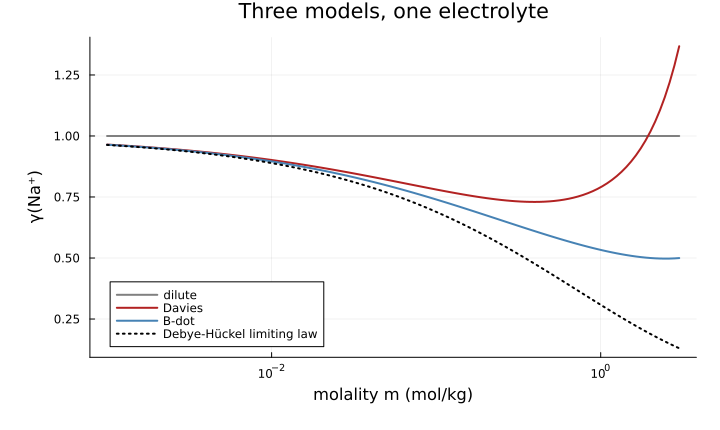
p2 = plot(; xscale = :log10, xlabel = "molality m (mol/kg)", ylabel = "water activity a_w",
    title = "The water activity barely separates", legend = :bottomleft)
for ((name, mod), col) in zip(models, (:gray, :firebrick, :steelblue))
    plot!(p2, ms, [aw(mod, m) for m in ms]; label = name, linewidth = 2, color = col,
        linestyle = name == "Davies" ? :dash : :solid)
end
plot(p2; size = (720, 430), left_margin = 10Plots.mm, bottom_margin = 8Plots.mm)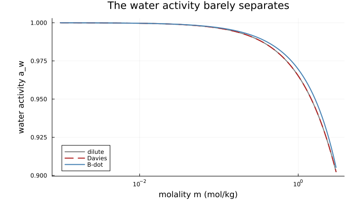
The ideal and Davies curves lie on top of each other in the second figure — both are Raoult — and the B-dot curve is a fraction of a percent away. A reader stopping here would conclude that the water-activity route is a detail. The next section is why that conclusion is wrong.
4. Gibbs-Duhem: the values agree, the derivatives do not
Equilibrium is set by chemical potentials, that is by derivatives of the activities with respect to composition — not by their values. So the test that matters is whether
M_W = 0.0180153
n_w = 1.0 / M_W
cs3 = ChemicalSystem([dict[s] for s in split("H2O@ Na+ Cl-")], ["H2O@", "Na+", "Cl-"])

function gd_residual(mod, m, dn)
    μ = build_potentials(cs3, mod)
    p = (ΔₐG⁰overRT = zeros(3), T = 298.15, P = 1.0e5, ϵ = 1.0e-30)
    n0 = [n_w, m, m]
    δ = 1.0e-6
    dμ = (μ(n0 + δ * dn, p) - μ(n0, p)) / δ
    return abs(sum(n0 .* dμ)) / max(norm(n0 .* abs.(dμ)), 1.0)
end

for (name, dn) in ("dissolution   dn = (0, +1, +1)" => [0.0, 1.0, 1.0],
                   "ion exchange  dn = (0, +1, -1)" => [0.0, 1.0, -1.0],
                   "water removal dn = (-1, 0, 0)" => [-1.0, 0.0, 0.0])
    println("\n── ", name)
    println("   m         dilute       Davies        B-dot")
    for m in (0.1, 0.3, 1.0, 3.0)
        r = [gd_residual(mod, m, dn) for (_, mod) in models]
        @printf("%6.2f    %10.3e   %10.3e   %10.3e\n", m, r...)
    end
end
── dissolution   dn = (0, +1, +1)
   m         dilute       Davies        B-dot
  0.10     2.934e-03    5.747e-02    1.100e-05
  0.30     8.793e-03    1.491e-02    2.516e-05
  1.00     2.907e-02    1.870e-01    6.702e-05
  3.00     8.508e-02    6.254e-01    1.082e-04

── ion exchange  dn = (0, +1, -1)
   m         dilute       Davies        B-dot
  0.10     7.071e-06    7.071e-06    9.004e-04
  0.30     2.357e-06    2.357e-06    2.041e-03
  1.00     7.072e-07    7.073e-07    4.276e-03
  3.00     2.355e-07    2.365e-07    6.954e-03

── water removal dn = (-1, 0, 0)
   m         dilute       Davies        B-dot
  0.10     1.294e-05    2.470e-04    2.527e-08
  0.30     1.156e-04    1.940e-04    2.656e-07
  1.00     1.253e-03    8.678e-03    2.552e-06
  3.00     1.054e-02    1.103e-01    1.492e-05
Three readings, and they are why this page exists.
Along a true dissolution, the B-dot model is four orders of magnitude more consistent than Davies. And Davies is worse than assuming ideality — not a paradox but the direct consequence of its construction: correcting the solutes while leaving the solvent at
Along an ion exchange at constant test/activities.jl uses, which is why its tolerance is 5e-3 and not solver tolerance.
Along water removal — the direction a drying paste takes — the ordering is the same as for dissolution, and the gap widens as the solution concentrates.
So the water-activity route is not a refinement on a number that hardly moves. It decides whether the model is one thermodynamic system or two halves that disagree, and only the derivatives show it.
p3 = plot(; xscale = :log10, yscale = :log10, xlabel = "molality m (mol/kg)",
    ylabel = "Gibbs-Duhem residual", legend = :topleft,
    title = "…and the derivatives separate by four orders")
mm = [0.03, 0.1, 0.3, 1.0, 3.0]
for ((name, mod), col) in zip(models, (:gray, :firebrick, :steelblue))
    μ = build_potentials(cs3, mod)
    r = [max(gd_residual(mod, m, [0.0, 1.0, 1.0]), 1.0e-16) for m in mm]
    plot!(p3, mm, r; label = name, linewidth = 2, color = col, marker = :circle)
end
plot(p3; size = (720, 430), left_margin = 10Plots.mm, bottom_margin = 8Plots.mm)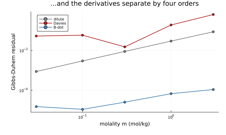
Along a dissolution, on a logarithmic axis: Davies sits above the ideal model at every molality, and the B-dot model below both by three to four orders.
What to take from this
below
DiluteSolutionModelis the best-conditioned objective;between there and about a molal, use
HKFActivityModel— and use it rather thanDaviesActivityModelwhenever the water activity enters the question, which in a hydrating paste it always does;above a few molal, none of the three is defensible, and no warning is issued because none of them knows.
solvent_fractionis the guard that does.
See also: Activity models for where the expressions come from, and Solid solution models for the same exercise on the mole-fraction side.