Titration of Malonic Acid by NaOH

This example simulates the potentiometric titration of malonic acid (H₂A, a diprotic weak acid) by sodium hydroxide (NaOH, a strong base). Both dissociation constants are derived from the database, not tabulated.

These species are malonate, not maleate

This page was titled "maleic acid" and drew maleic acid's tabulated constants (pKₐ₁ = 1.92, pKₐ₂ = 6.27) over a curve computed from malonate data — so the two dotted lines crossed the curve at neither half-equivalence point, which was visible in the published figure. SLOP98 names the three species MALONIC-ACID,AQ, H-MALONATE,AQ and MALONATE,AQ, and their formula carries three carbons: malonic acid is HOOC–CH₂–COOH (propanedioic acid, C₃H₄O₄), whereas maleic acid is the cis-butenedioic acid C₄H₄O₄. Neither maleic nor fumaric acid is present in SLOP98. The constants derived below agree with the accepted values for malonic acid to 0.02.

System setup

The species are distributed across two SLOP98 databases: the inorganic database provides H₂O, H⁺, OH⁻ and Na⁺; the organic database provides malonic acid and its conjugate bases.

Symbol	Species	Phase
`MalH2@`	H₂A — malonic acid	aqueous solute
`MalH-`	HA⁻ — hydrogen malonate	aqueous solute
`Mal-2`	A²⁻ — malonate	aqueous solute
`Na+`	Na⁺	aqueous solute
`H+`	H⁺	aqueous solute
`OH-`	OH⁻	aqueous solute
`H2O@`	H₂O	aqueous solvent

julia

using ChemistryLab
using DynamicQuantities

substances_inorg = build_species(datapath("slop98-inorganic-thermofun.json"))
substances_org   = build_species(datapath("slop98-organic-thermofun.json"))

dict_all_species = merge(Dict(symbol(s) => s for s in substances_inorg), Dict(symbol(s) => s for s in substances_org))
species = [dict_all_species[s] for s in split("H2O@ Na+ NaOH@ H+ OH- MalH2@ MalH- Mal-2")]

cs = ChemicalSystem(species, ["H2O@", "H+", "Mal-2", "Na+", "Zz"])

┌──────────────────────────────────────────────────────────┐
│  Loading database: data/slop98-inorganic-thermofun.json  │
└──────────────────────────────────────────────────────────┘
┌────────────────────┐
│  Building species  │
└────────────────────┘

Progress:  23%|█████████████████████████████████████▏                                                                                                                           |  ETA: 0:00:00[K
Progress:  47%|███████████████████████████████████████████████████████████████████████████                                                                                      |  ETA: 0:00:00[K
Progress:  70%|████████████████████████████████████████████████████████████████████████████████████████████████████████████████▌                                                |  ETA: 0:00:00[K
Progress:  93%|█████████████████████████████████████████████████████████████████████████████████████████████████████████████████████████████████████████████████████▊           |  ETA: 0:00:00[K
Progress:  99%|████████████████████████████████████████████████████████████████████████████████████████████████████████████████████████████████████████████████████████████████▉|  ETA: 0:00:00[K
Progress: 100%|█████████████████████████████████████████████████████████████████████████████████████████████████████████████████████████████████████████████████████████████████| Time: 0:00:00[K
┌────────────────────────────────────────────────────────┐
│  Loading database: data/slop98-organic-thermofun.json  │
└────────────────────────────────────────────────────────┘
┌────────────────────┐
│  Building species  │
└────────────────────┘

Progress:  39%|███████████████████████████████████████████████████████████████▌                                                                                                 |  ETA: 0:00:00[K
Progress:  79%|██████████████████████████████████████████████████████████████████████████████████████████████████████████████████████████████▊                                  |  ETA: 0:00:00[K
Progress: 100%|█████████████████████████████████████████████████████████████████████████████████████████████████████████████████████████████████████████████████████████████████| Time: 0:00:00[K

The two constants come from the database

Both are computed from the standard Gibbs energies of formation the database ships. The literature values are printed for comparison and never enter the calculation.

julia

R  = ustrip(Constants.R)
T  = 298.15   # K
RT = R * T

sp = Dict(symbol(s) => s for s in cs.species)

# MalH2@ ⇌ MalH⁻ + H⁺
Ka1  = exp(-(sp["MalH-"].ΔₐG⁰(T = T) + sp["H+"].ΔₐG⁰(T = T) - sp["MalH2@"].ΔₐG⁰(T = T)) / RT)
pKa1 = -log10(Ka1)

# MalH⁻ ⇌ Mal²⁻ + H⁺
Ka2  = exp(-(sp["Mal-2"].ΔₐG⁰(T = T) + sp["H+"].ΔₐG⁰(T = T) - sp["MalH-"].ΔₐG⁰(T = T)) / RT)
pKa2 = -log10(Ka2)

println("pKa1 (MalH2@ / MalH⁻) = ", round(pKa1, digits = 2), "   (lit. malonic 2.83)")
println("pKa2 (MalH⁻  / Mal²⁻) = ", round(pKa2, digits = 2), "   (lit. malonic 5.69)")
println("Δ pKa                 = ", round(pKa2 - pKa1, digits = 2))

pKa1 (MalH2@ / MalH⁻) = 2.85   (lit. malonic 2.83)
pKa2 (MalH⁻  / Mal²⁻) = 5.7   (lit. malonic 5.69)
Δ pKa                 = 2.84

Build the EquilibriumSolver once — it is reused at every titration point:

julia

using Optimization, OptimizationIpopt

solver = EquilibriumSolver(
    cs,
    DiluteSolutionModel(),
    IpoptOptimizer(
        mu_strategy = "adaptive",
    );
    variable_space = Val(:linear),
    abstol  = 1e-8,
    reltol  = 1e-8,
    maxiters = 100,
    verbose = false,
)

Running the titration

At each titration point the total composition is reset from scratch and the equilibrium is recomputed. The conservation constraint (total moles of each component) is enforced by the solver.

julia

V_acid = 100e-3   # volume of acid solution, L
c_acid = 0.1      # malonic acid concentration, mol/L
c_base = 2.0      # NaOH concentration, mol/L
n_H2A  = V_acid * c_acid   # total moles of H₂A = 10 mmol

ρ_water = 1.0   # kg/L

V_eq1 = n_H2A / c_base * 1e3       # first equivalence point,  5 mL
V_eq2 = 2 * n_H2A / c_base * 1e3   # second equivalence point, 10 mL

volumes_NaOH = collect(range(0, 15; length = 101))   # mL, step 0.15 mL
pH_vals = Float64[]

s = ChemicalState(cs)
for V_mL in volumes_NaOH
    V_NaOH  = V_mL * 1e-3            # L
    n_NaOH  = c_base * V_NaOH        # mol of NaOH (= mol of Na⁺ added)
    V_total = V_acid + V_NaOH        # total volume, L

    set_quantity!(s, "MalH2@", n_H2A * u"mol")
    set_quantity!(s, "NaOH@", n_NaOH * u"mol")
    set_quantity!(s, "H2O@",  ρ_water * V_total * u"kg")

    V_liq = volume(s).liquid
    set_quantity!(s, "H+",  1e-7u"mol/L" * V_liq)   # pH-neutral seed
    set_quantity!(s, "OH-", 1e-7u"mol/L" * V_liq)

    s_eq = solve(solver, s)
    push!(pH_vals, pH(s_eq))
end

# Indices are looked up from the volume, never hard-coded.
at(V) = argmin(abs.(volumes_NaOH .- V))

for (V, what) in ((0.0, "pure acid"), (V_eq1 / 2, "½ PE₁"), (V_eq1, "PE₁"),
                  (V_eq1 + V_eq1 / 2, "½ PE₂"), (V_eq2, "PE₂"), (15.0, "excess NaOH"))
    i = at(V)
    println("pH at V = ", lpad(round(volumes_NaOH[i], digits = 2), 5), " mL  ",
            rpad("($what)", 15), " : ", round(pH_vals[i], digits = 2))
end

┌ Warning: equilibrium solve returned `Failure`; the composition may not be an equilibrium. Set `ChemistryLab.STRICT_CONVERGENCE[] = true` to raise instead.
└ @ ChemistryLab ~/work/ChemistryLab.jl/ChemistryLab.jl/src/equilibrium/equilibrium_solver.jl:398
pH at V =   0.0 mL  (pure acid)     : 1.96
pH at V =  2.55 mL  (½ PE₁)         : 2.89
pH at V =  4.95 mL  (PE₁)           : 4.22
pH at V =   7.5 mL  (½ PE₂)         : 5.7
pH at V = 10.05 mL  (PE₂)           : 10.9
pH at V =  15.0 mL  (excess NaOH)   : 12.87

The two half-equivalence points return the two constants, which is the Henderson–Hasselbalch condition and the internal check the previous version of this page failed.

Titration curve

julia

using Plots

p = plot(
    volumes_NaOH, pH_vals;
    xlabel     = "V(NaOH) (mL)",
    ylabel     = "pH",
    label      = "Titration curve",
    linewidth  = 2,
    marker     = :circle,
    markersize = 3,
    color      = :steelblue,
    title      = "Titration of malonic acid (0.1 M) by NaOH (2 M)",
    ylims      = (0, 14),
    legend     = :topleft,
)
vline!(p, [V_eq1]; linestyle = :dash, color = :red,    label = "PE₁ ($(round(V_eq1, digits = 1)) mL)")
vline!(p, [V_eq2]; linestyle = :dash, color = :blue,   label = "PE₂ ($(round(V_eq2, digits = 1)) mL)")
hline!(p, [pKa1];  linestyle = :dot,  color = :orange, label = "pKₐ₁ = $(round(pKa1, digits = 2)) (from the database)")
hline!(p, [pKa2];  linestyle = :dot,  color = :green,  label = "pKₐ₂ = $(round(pKa2, digits = 2)) (from the database)")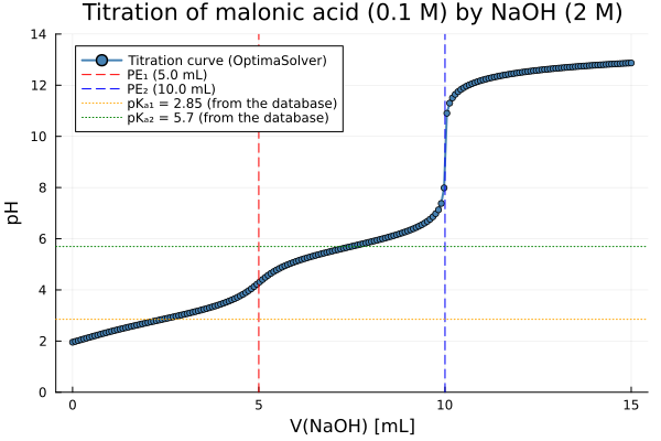

Analysis

Zone	V(NaOH)	Dominant species	pH
Initial state	0 mL	H₂A	Low, controlled by pKₐ₁
First buffer	0–5 mL	H₂A / HA⁻	≈ pKₐ₁ at V = 2.5 mL
First equivalence point (PE₁)	5 mL	HA⁻	First inflection
Second buffer	5–10 mL	HA⁻ / A²⁻	≈ pKₐ₂ at V = 7.5 mL
Second equivalence point (PE₂)	10 mL	A²⁻	Second inflection
Excess base	> 10 mL	A²⁻ + OH⁻	Controlled by excess NaOH

V = 0 mL — the pH is low, determined mainly by the first dissociation.
V = 2.5 mL (half-equivalence 1) — pH ≈ pKₐ₁, the Henderson–Hasselbalch condition.
V = 5 mL (PE₁) — the first proton is neutralized; the dominant species goes from H₂A to HA⁻.
5 mL < V < 10 mL — the HA⁻/A²⁻ couple buffers; at V = 7.5 mL, pH ≈ pKₐ₂.
V = 10 mL (PE₂) — the second proton is neutralized; the dominant species is A²⁻.
V > 10 mL — the pH rises steeply, controlled by free OH⁻ from the excess NaOH.

Δ pKₐ and how well the first equivalence point resolves

The two constants of malonic acid are separated by Δ pKₐ ≈ 2.85. That is enough for two distinguishable buffer regions, but not enough for a sharp first equivalence point: at V = 5 mL the curve shows a gentle inflection rather than a jump, and only the second equivalence point rises steeply. An earlier version of this page claimed "Δ pKₐ ≈ 4.35 … two clearly resolved inflection points" — that figure belongs to maleic acid, and the claim does not survive looking at the curve it accompanied.

Titration of Malonic Acid by NaOH ​

System setup ​

The two constants come from the database ​

Running the titration ​

Titration curve ​

Analysis ​

Titration of Malonic Acid by NaOH

System setup

The two constants come from the database

Running the titration

Titration curve

Analysis