Bogue Calculation

Before this page

Cement chemist notation and Stoichiometric Matrix.

The way in which species and cementitious species are constructed in ChemistryLab and expressed as a linear combination of reference species opens the door to equilibrium calculations. It also makes it quite natural to retrieve Bogue's formulas and use them simply.

Bogue's formulas allow us to find the masses of , , and as a function of the oxides (, , and ) that are regularly found in manufacturers' cement data sheets. However, using the StoichMatrix functions performs a molar decomposition of the species that we wish to decompose as a function of reference species. It is therefore possible to express the anhydrous of the cement as a function of the oxides in a cement data sheet.

Via ChemicalSystem

The recommended approach builds a ChemicalSystem once, which computes both stoichiometric matrices and all derived structures automatically. The four clinker phases are the species; the four oxide components (C=, S=, A=, F=) are the primaries:

cemspecies = CemSpecies.(split("C3S C2S C3A C4AF"))
oxides = CemSpecies.(split("C S A F"))

cs = ChemicalSystem(cemspecies, oxides)
A = cs.SM.A

4×4 Matrix{Int64}:
 3  2  3  4
 1  1  0  0
 0  0  1  1
 0  0  0  1

The stoichiometric matrix cs.SM.A (primaries × species) gives the molar decomposition of each clinker phase into oxides. Bogue's formulas are obtained by converting to mass and inverting:

# Molar mass of anhydrous phases
Mw  = map(x -> ustrip(us"g/mol", x.M), cemspecies)
# Molar mass of each oxide
Mwo = map(x -> ustrip(us"g/mol", x.M), oxides)
Aoa = Mwo .* A .* inv.(Mw)'

pprint(inv(Aoa), cemspecies, oxides; label=:name)

┌──────┬─────────────────────┬────────────────────┬────────────────────┬─────────────────────┐
│      │                   C │                  S │                  A │                   F │
├──────┼─────────────────────┼────────────────────┼────────────────────┼─────────────────────┤
│  C3S │   4.071437487740072 │ -7.599953397799711 │ -6.717746999578564 │ -1.4297594669572347 │
│  C2S │ -3.0714374877400723 │  8.599953397799712 │  5.067777665699052 │  1.0785912441213124 │
│  C3A │                     │                    │ 2.6499693338795134 │ -1.6920042132421553 │
│ C4AF │                     │                    │                    │   3.043172436078078 │
└──────┴─────────────────────┴────────────────────┴────────────────────┴─────────────────────┘

By taking a cement sheet with classic percentages of oxides (=65.6%, =21.5%, =5.2% and =2.8%), we obtain the anhydrous mass fractions of the cementitious material:

inv(Aoa) * [65.6, 21.5, 5.2, 2.8]

4-element Vector{Float64}:
 64.75169023776614
 12.785198202119847
  9.042228739095435
  8.520882821018617

The analysis in, and the clinker phases out, both in percent by mass:

using Plots
oxide_percent = [65.6, 21.5, 5.2, 2.8]
phase_percent = inv(Aoa) * oxide_percent
p_in = bar(["CaO", "SiO₂", "Al₂O₃", "Fe₂O₃"], oxide_percent; legend = false, color = :grey60,
           ylabel = "% by mass", title = "The oxide analysis", titlefontsize = 10)
p_out = bar(["C₃S", "C₂S", "C₃A", "C₄AF"], phase_percent; legend = false, color = :steelblue,
            title = "Bogue's phases", titlefontsize = 10)
plot(p_in, p_out; layout = (1, 2), size = (760, 340), ylims = (0, 72), framestyle = :box, grid = false,
     left_margin = 5Plots.mm, bottom_margin = 5Plots.mm)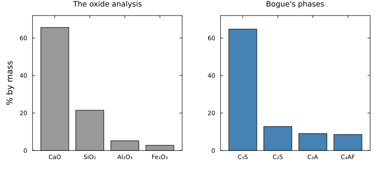

---

Via mass_matrix

A more direct route uses mass_matrix on the canonical stoichiometric matrix. This expresses each species as a linear combination of the reference oxide components directly in mass rather than in moles, making Bogue's formulas immediate:

massCSM = mass_matrix(CanonicalStoichMatrix(cemspecies))
pprint(inv(massCSM.A), cemspecies, oxides; label=:name)

┌──────┬────────────────────┬─────────────────────┬────────────────────┬─────────────────────┐
│      │                  C │                   S │                  A │                   F │
├──────┼────────────────────┼─────────────────────┼────────────────────┼─────────────────────┤
│  C3S │  4.071437487740072 │ -7.5999533977997125 │ -6.717746999578565 │ -1.4297594669572344 │
│  C2S │ -3.071437487740072 │   8.599953397799712 │  5.067777665699052 │  1.0785912441213117 │
│  C3A │                    │                     │  2.649969333879514 │ -1.6920042132421553 │
│ C4AF │                    │                     │                    │  3.0431724360780774 │
└──────┴────────────────────┴─────────────────────┴────────────────────┴─────────────────────┘

Where to go next

The matrix inverted here is examined for itself in Stoichiometric matrices. The phase masses obtained are the starting point of A CEM I from its clinker phases.