Chemical Equilibrium

Before this page

Getting started, and the Manual pages on Species and on ChemicalSystem and ChemicalState. Why the calculation is the right one is explained in Thermochemistry.

ChemistryLab computes a thermodynamic equilibrium as the minimum of the Gibbs energy under the element-conservation constraints, and the workflow always follows the same four steps:

1. Build a ChemicalSystem (species + stoichiometric matrix).

2. Create an initial ChemicalState (temperature, pressure, initial amounts).

3. Call equilibrate (or use EquilibriumSolver explicitly).

4. Inspect the resulting ChemicalState.

Minimal workflow

The convenience function equilibrate handles everything with sensible defaults. The example below computes the equilibrium state of calcite (CaCO₃) dissolving in mildly acidic water — a standard geochemical benchmark.

using Optimization, OptimizationIpopt
using ChemistryLab
using DynamicQuantities

substances = build_species(datapath("slop98-inorganic-thermofun.json"); verbose = false)

# Select the carbonate-system species, calcite and its dissolution product Ca²⁺
dict = Dict(symbol(s) => s for s in substances)
species = [dict[sym] for sym in split("H2O@ H+ OH- CO2@ HCO3- CO3-2 Ca+2 Cal")]

cs = ChemicalSystem(species, ["H2O@", "H+", "Ca+2", "CO3-2", "Zz"])

The chemical system in full

cs

8-element ChemicalSystem{Species{Int64}, AbstractReaction, StoichMatrix{Int64, Symbol, Vector{Symbol}, Matrix{Int64}, Species{Int64}}, StoichMatrix{Int64, Species{Int64}, Vector{Species{Int64}}, Matrix{Int64}, Species{Int64}}, Nothing, Nothing}:
 H2O@ {Water HGK} [H2O@ ◆ H₂O@]
 H+ {H+} [H+ ◆ H⁺]
 OH- {OH- hydroXyl ion} [OH- ◆ OH⁻]
 CO2@ {CO2,aq (+ H2O = H2CO3,aq )} [CO2@ ◆ CO₂@]
 HCO3- {HCO3- bicarbonate ion} [HCO3- ◆ HCO₃⁻]
 CO3-2 {CO3-2 carbonate ion} [CO3-2 ◆ CO₃²⁻]
 Ca+2 {Ca+2 ion} [Ca+2 ◆ Ca²⁺]
 Cal {CALCITE} [CaCO3 ◆ CaCO₃]

state = ChemicalState(cs)

# 1 mmol calcite dissolved in 1 L of acidic water (initial pH ≈ 4)
set_quantity!(state, "Cal",  1e-3u"mol")
set_quantity!(state, "H2O@", 1.0u"kg")

V = volume(state)
set_quantity!(state, "H+",  1e-4u"mol/L" * V.liquid)   # pH = 4
set_quantity!(state, "OH-", 1e-10u"mol/L" * V.liquid)  # charge seed

state_eq = equilibrate(state)

The solved state in full — every species, with its amount

state_eq

ChemicalState{Species{Int64}, AbstractReaction, Quantity{Float64, SymbolicDimensions{FRInt32}}, Float64}
┌────────────────────────────────────────────────────────────────────────────────────────────────┐
│           T : 298.15 K                                                                         │
│           P : 1.0 bar                                                                          │
╞════════════════════════════════════════════════════════════════════════════════════════════════╡
│  # liquid #│             n [mol]│               m [g]│             V [cm³]│           c [mol/L]│
├┄┄┄┄┄┄┄┄┄┄┄┄┄┄┄┄┄┄┄┄┄┄┄┄┄┄┄┄┄┄┄┄┄┄┄┄┄┄┄┄┄┄┄┄┄┄┄┄┄┄┄┄┄┄┄┄┄┄┄┄┄┄┄┄┄┄┄┄┄┄┄┄┄┄┄┄┄┄┄┄┄┄┄┄┄┄┄┄┄┄┄┄┄┄┄┄┤
│ tot. liquid│             55.5096│             1000.02│             1002.95│                    │
├┄┄┄┄┄┄┄┄┄┄┄┄┄┄┄┄┄┄┄┄┄┄┄┄┄┄┄┄┄┄┄┄┄┄┄┄┄┄┄┄┄┄┄┄┄┄┄┄┄┄┄┄┄┄┄┄┄┄┄┄┄┄┄┄┄┄┄┄┄┄┄┄┄┄┄┄┄┄┄┄┄┄┄┄┄┄┄┄┄┄┄┄┄┄┄┄┤
│        H2O@│             55.5093│             999.999│             1002.95│             55.3462│
│        Ca+2│         0.000155619│           0.0062369│         -0.00286942│         0.000155162│
│       HCO3-│         0.000134259│          0.00819192│          0.00325052│         0.000133864│
│         OH-│          3.41402e-5│         0.000580622│        -0.000160726│          3.40399e-5│
│       CO3-2│          2.12725e-5│          0.00127652│        -0.000128863│            2.121e-5│
│        CO2@│          8.79438e-8│          3.87032e-6│          2.88514e-6│          8.76854e-8│
│          H+│          2.9603e-10│         2.98398e-10│                 0.0│          2.9516e-10│
╞════════════════════════════════════════════════════════════════════════════════════════════════╡
│   # solid #│             n [mol]│               m [g]│             V [cm³]│                    │
├┄┄┄┄┄┄┄┄┄┄┄┄┄┄┄┄┄┄┄┄┄┄┄┄┄┄┄┄┄┄┄┄┄┄┄┄┄┄┄┄┄┄┄┄┄┄┄┄┄┄┄┄┄┄┄┄┄┄┄┄┄┄┄┄┄┄┄┄┄┄┄┄┄┄┄┄┄┄┄┄┄┄┄┄┄┄┄┄┄┄┄┄┄┄┄┄┤
│  tot. solid│         0.000844381│           0.0845107│           0.0311864│                    │
├┄┄┄┄┄┄┄┄┄┄┄┄┄┄┄┄┄┄┄┄┄┄┄┄┄┄┄┄┄┄┄┄┄┄┄┄┄┄┄┄┄┄┄┄┄┄┄┄┄┄┄┄┄┄┄┄┄┄┄┄┄┄┄┄┄┄┄┄┄┄┄┄┄┄┄┄┄┄┄┄┄┄┄┄┄┄┄┄┄┄┄┄┄┄┄┄┤
│         Cal│         0.000844381│           0.0845107│           0.0311864│                    │
╞════════════════════════════════════════════════════════════════════════════════════════════════╡
│   # TOTAL #│             n [mol]│               m [g]│             V [cm³]│                    │
├┄┄┄┄┄┄┄┄┄┄┄┄┄┄┄┄┄┄┄┄┄┄┄┄┄┄┄┄┄┄┄┄┄┄┄┄┄┄┄┄┄┄┄┄┄┄┄┄┄┄┄┄┄┄┄┄┄┄┄┄┄┄┄┄┄┄┄┄┄┄┄┄┄┄┄┄┄┄┄┄┄┄┄┄┄┄┄┄┄┄┄┄┄┄┄┄┤
│            │             55.5105│              1000.1│             1002.98│                    │
╞════════════════════════════════════════════════════════════════════════════════════════════════╡
│          pH : 9.5274                                                                           │
│         pOH : 4.468                                                                            │
│    porosity : 0.999969                                                                         │
│  saturation : 1.0                                                                              │
└────────────────────────────────────────────────────────────────────────────────────────────────┘

Quick shortcut

Calling equilibrate(state) with no extra arguments uses sensible defaults and is usually sufficient for aqueous geochemical problems.

The call above does more than it shows. equilibrate starts from every interior-point back end that is loaded — Ipopt, and the one OptimaSolver provides — refines each answer with the dual Newton method of OptimaSolver, and returns the answer whose optimality it can prove. Which back ends exist, how they compare and how one of them is imposed are described in Solving an equilibrium, together with the constraints other than a fixed temperature and pressure, the differentiation of an equilibrium with respect to its inputs, the activity models and the declaration of solid solutions. This tutorial keeps to the calculation itself.

Certifying an answer

equilibrate takes the certifying route by default, and it returns a composition together with a proof that it is the Gibbs minimum rather than the point an iteration stopped at. Why such a proof exists — the problem is convex, so the KKT conditions are sufficient and not merely necessary — what the three conditions are, and how DualEquilibriumSolver aims at them directly, are in Proving that an answer is the answer.

A solver passed explicitly runs that one back end and hands its answer to the dual Newton, which polishes it; certificate receives the proof of what is returned. The dual Newton can also be driven on its own, from a composition obtained elsewhere:

cert = Ref{Any}()
eq   = equilibrate(state, OptimaOptimizer(); certificate = cert)
cert[].optimal  # true: a proof, for a convex problem

des  = DualEquilibriumSolver(cs, HKFActivityModel())
dual = solve(des, start; b = b)                   # to the KKT conditions
optimality_certificate(des, dual; b = b).optimal

Inspecting the equilibrium state

The returned ChemicalState carries all derived thermodynamic quantities:

println("pH      = ", pH(state_eq))
println("pOH     = ", pOH(state_eq))
println("porosity   = ", porosity(state_eq))
println("saturation = ", saturation(state_eq))

pH      = 9.527382810745273
pOH     = 4.468012228308951
porosity   = 0.9999689062319774
saturation = 1.0

Phase volumes and mole amounts are accessible via named tuples:

v = volume(state_eq)
println("V liquid = ", v.liquid)
println("V solid  = ", v.solid)
println("V total  = ", v.total)

m = moles(state_eq)
println("n liquid = ", m.liquid)
println("n solid  = ", m.solid)

V liquid = 0.0010029467739939588 m³
V solid  = 3.1186364031165686e-8 m³
V total  = 0.00100297796035799 m³
n liquid = 55.509609153069746 mol
n solid  = 0.000844380917949484 mol

Individual species amounts (in mol):

cs_eq = state_eq.system
for (i, sp) in enumerate(cs_eq.species)
    n_i = state_eq.n[i]
    println(rpad(symbol(sp), 20), ustrip(n_i), " mol")
end

H2O@                55.50926377444133 mol
H+                  2.960302339984174e-10 mol
OH-                 3.414016828141692e-5 mol
CO2@                8.79437736049244e-8 mol
HCO3-               0.00013425861384723045 mol
CO3-2               2.127252442968135e-5 mol
Ca+2                0.0001556190820505154 mol
Cal                 0.000844380917949484 mol

Scaling and normalization

It is often useful to express a composition relative to a reference amount — per mole, per kilogram, or per cubic meter of system. Two mechanisms are provided.

Scalar multiplication

A ChemicalState can be multiplied or divided by a real number. All molar amounts are scaled proportionally; temperature, pressure, and the chemical system are unchanged. The operation is non-mutating — a new state is returned:

state2  = state_eq * 2.0    # double all amounts
state_m = state_eq / 1000   # millimolar scale

rescale! — rescale to a target total

rescale! scales all molar amounts in-place so that the total of the matching physical quantity equals target:

target dimension	Quantity brought to target
mol	moles(state).total
kg (mass)	mass(state).total
m³ (volume)	volume(state).total

All derived quantities (pH, porosity, volume, …) are recomputed automatically after scaling.

# Express the equilibrium composition per kilogram of total system
state_pkg = copy(state_eq)
rescale!(state_pkg, 1.0u"kg")

println("Ca²⁺ = ", moles(state_pkg, "Ca+2"), "  mol/kg")
println("pH   = ", pH(state_pkg))   # intensive quantities are invariant

Ca²⁺ = 0.0001556034925880364 mol  mol/kg
pH   = 9.527382810745273

Intensive quantities

pH, porosity, and saturation are intensive — they are invariant under homothety and remain unchanged after rescale! or scalar multiplication.

Using EquilibriumSolver explicitly

For batch calculations where many different initial states share the same system and activity model, construct an EquilibriumSolver once and reuse it:

using Optimization, OptimizationIpopt

opt = IpoptOptimizer(
    acceptable_tol        = 1e-12,
    dual_inf_tol          = 1e-12,
    acceptable_iter       = 1000,
    constr_viol_tol       = 1e-12,
    warm_start_init_point = "no",
    additional_options    = Dict{String, Any}("print_level" => 0, "sb" => "yes"),
)

solver = EquilibriumSolver(
    cs,
    DiluteSolutionModel(),
    opt;
    variable_space = Val(:linear),
    reltol  = 1e-10,
)

Ipopt prints an iteration table for every solve unless told otherwise; print_level = 0 and sb = "yes" (no banner) keep it silent, and the default solver of equilibrate is built the same way. reltol becomes Ipopt's convergence tolerance tol.

Once built, solver is called with any compatible ChemicalState:

state_eq2 = solve(solver, state)
println("pH = ", round(pH(state_eq2); digits = 4), ", as from `equilibrate`: ", round(pH(state_eq); digits = 4))

pH = 9.5274, as from `equilibrate`: 9.5274

Performance

The potential function μ(n, p) is compiled once during EquilibriumSolver construction. Repeated calls to solve(solver, ...) with different states reuse it, avoiding redundant compilation overhead.

Temperature dependence (10–30 °C)

Calcite solubility varies with temperature. Using the solver built above, we sweep from 10 to 30 °C and track pH, dissolved calcium and remaining solid calcite:

using Plots


temperatures = 10:30   # °C

pH_vals   = Float64[]
nCa_vals  = Float64[]  # mmol
nCal_vals = Float64[]  # mmol

i_Ca  = findfirst(sp -> symbol(sp) == "Ca+2", cs.species)
i_Cal = findfirst(sp -> symbol(sp) == "Cal",  cs.species)

# Start from the charged state built above, not from `ChemicalState(cs)`:
# a fresh state holds no matter at all, so every element balance would be zero
# and the sweep would return the same trivial solution at all 21 temperatures.
for θ in temperatures
    s_T = deepcopy(state)
    set_temperature!(s_T, (273.15 + θ) * u"K")
    s_eq = solve(solver, s_T)
    push!(pH_vals,   pH(s_eq))
    push!(nCa_vals,  ustrip(s_eq.n[i_Ca]) * 1e3)
    push!(nCal_vals, ustrip(s_eq.n[i_Cal]) * 1e3)
end

The figures can then be drawn.

p1 = plot(collect(temperatures), pH_vals,
    xlabel = "T (°C)", ylabel = "pH", label = "pH",
    marker = :circle, linewidth = 2, title = "pH")
p2 = plot(collect(temperatures), nCa_vals,
    xlabel = "T (°C)", ylabel = "n (mmol)", label = "Ca²⁺",
    marker = :circle, linewidth = 2, title = "Dissolved species")
plot!(p2, collect(temperatures), nCal_vals,
    label = "Cal", marker = :square, linewidth = 2)
plot(p1, p2, layout = (1, 2), left_margin = 8Plots.mm, bottom_margin = 8Plots.mm, size = (900, 400))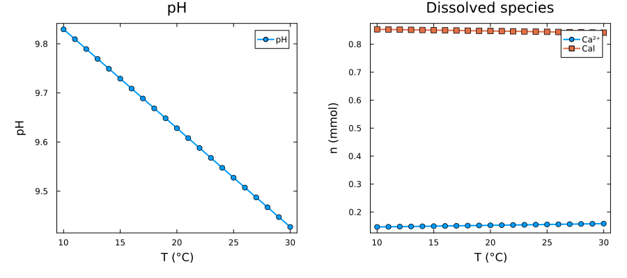

Retrograde Kₛₚ, and yet more dissolved calcium

Calcite is retrograde soluble: its solubility product falls as temperature rises. The sweep above reproduces that — the ionic product it settles on goes from at 10 °C to at 30 °C, matching the the database itself gives to within 0.003 log units, and at 25 °C is the accepted value for calcite.

The dissolved calcium nevertheless increases, from 0.146 to 0.158 mmol/L. That is not a contradiction: this system is closed, with 1 mmol of total carbonate and no CO₂ reservoir. As temperature rises the pH drops from 9.83 to 9.43, which shifts carbonate to bicarbonate and takes free CO₃²⁻ from 26.5 down to 19.2 µmol/L — more than enough to offset the smaller . The familiar statement that retrograde solubility means less dissolved calcium holds for a system buffered at a fixed CO₂ partial pressure, not for a sealed one. Fix the partial pressure instead (add a gas phase) and the sign flips.

Reading the aqueous properties back

The activity model used so far is the default, DiluteSolutionModel; the others, and the reasons for choosing one, are in Activity models (syntax) and Activity models (theory). Whatever the model, the quantities it computes can be read back from a state.

The activity closures compute the molalities, the ionic strength and the activity coefficients on their way to the log-activities. All of it is readable off a state:

call	returns
molalities(state)	mᵢ of every solute, mol/kg of solvent
ionic_strength(state)	I = ½ Σ mⱼ zⱼ², mol/kg
activity_coefficients(state, model)	γᵢ of every aqueous species
log_activities(state, model)	ln aᵢ of every species
activities(state, model)	aᵢ of every species
pH(state, model)	−log₁₀ a(H⁺)
pOH(state, model)	−log₁₀ a(OH⁻)

eq = equilibrate(state; model = HKFActivityModel())

ionic_strength(eq)                      # 0.212 mol/kg
molalities(eq)["K+"]                    # 0.146 mol/kg
activity_coefficients(eq, model)["Ca+2"]
activities(eq, model)["H2O@"]           # water activity
pH(eq, model)                           # activity convention

molalities and ionic_strength need no model: they are properties of the composition, and every model in the package computes the ionic strength this way. When comparing against another code, compare the ionic strength first — if it disagrees, the two are not describing the same solution, whatever their volumes happen to agree on.

Two conventions of pH, 0.2 units apart

The one-argument pH(state) and the two-argument pH(state, model) are different quantities:

• pH(state) is −log₁₀ c(H⁺), a concentration in mol/L over the computed liquid volume, and in an alkaline solution it is reconstructed from OH⁻ through pKw. It is stored on the state and needs no activity model.

• pH(state, model) is −log₁₀ a(H⁺), the activity on the molality scale. This is what GEM-Selektor (Kulik et al., 2013), PHREEQC (Parkhurst and Appelo, 2013) and Reaktoro (Leal et al., 2017) report.

On a Portland cement pore solution at I ≈ 0.2 mol/kg, with γ(H⁺) ≈ 0.61, the two differ by about 0.21 units (13.31 against 13.10). Comparing the wrong one against another code means chasing a discrepancy that is a convention, not a result.

γ comes from the formula, not from a ratio

activity_coefficients evaluates the model's own expression, rather than dividing an activity by a concentration. The ratio agrees for an abundant solute — the test suite checks that it does — but a species parked at the solver's 1e-16 mol lower bound has its log-activity dominated by the closures' + ϵ regularization, and the ratio then returns values of order 1e300 for a charge class whose only members are trace. The formula depends on the ionic strength and the charge alone, so it is exact at any amount.

Relatedly, an activity is a number on a scale, and nothing in the number says which. DiluteSolutionModel puts its solutes on the molarity scale and takes ρ = 1 kg/L, so its activities coincide numerically with molalities even though the scale differs; the other two models are on the molality scale. concentration_scale is the only way to tell them apart.

Where to go next

The options this tutorial left at their defaults are gathered in Solving an equilibrium. The application pages then apply the same four steps to systems of increasing size: the aqueous cases, beginning with CO₂ dissolution and the carbonate system, are small enough to check by hand, and A CEM I from its clinker phases is the first cement. When the question is how a system evolves in time rather than where it ends, the next tutorial is Chemical Kinetics.