
Cement clinker hydration kinetics
This example demonstrates the full kinetics workflow: from database loading to ODE integration and calorimetric post-processing. It models the hydration of an OPC (CEM I 52.5 R) clinker using the Parrot–Killoh (Parrott and Killoh, 1984) rate model with Arrhenius temperature correction (Schindler and Folliard, 2005), coupled to a semi-adiabatic calorimeter (Lavergne et al., 2018).
1. Chemical system
We select the four clinker phases as kinetic species, plus the main hydration products and water. CEMDATA_PRIMARIES provides the independent aqueous components.
using ChemistryLab
using OrdinaryDiffEq
using DynamicQuantities
using OrderedCollections

DATA_FILE = datapath("cemdata18-thermofun.json")

substances = build_species(DATA_FILE)

input_species = split(
    "C3S C2S C3A C4AF " *
        "Portlandite Jennite ettringite monosulphate12 C3AH6 C3FH6 " *
        "H2O@",
)

species = speciation(substances, input_species; aggregate_state = [AS_AQUEOUS])
cs = ChemicalSystem(species, CEMDATA_PRIMARIES)

println("Chemical system: $(length(cs.species)) species")
┌───────────────────────────────────────────────────┐
│ Loading database: data/cemdata18-thermofun.json │
└───────────────────────────────────────────────────┘
┌────────────────────┐
│ Building species │
└────────────────────┘
Progress: 82%|███████████████████████████████████████████████████████████████████████████████████████████████████████████████████████████████████▍ | ETA: 0:00:00[K
Progress: 100%|█████████████████████████████████████████████████████████████████████████████████████████████████████████████████████████████████████████████████████████████████| Time: 0:00:00[K
Chemical system: 51 species2. Initial state
Typical CEM I 52.5 R composition from (Lavergne et al., 2018). We work with 1 kg of cement at water/cement ratio
const WC = 0.4
const COMPOSITION = (C3S = 0.619, C2S = 0.165, C3A = 0.08, C4AF = 0.087)

state0 = ChemicalState(cs)
for (name, frac) in pairs(COMPOSITION)
    set_quantity!(state0, string(name), frac * u"kg")
end
set_quantity!(state0, "H2O@", WC * u"kg")
3. Parrot–Killoh kinetic models
Maximum degree of hydration from the (Powers, 1948) law:
This uses parrot_killoh_avrami with PK84_PARAMS_*, the canonical formulation. The smoothed parrot_killoh variant this page used until v0.14.0 is deprecated: it is diffusion-limited from a few percent of hydration on, which held the mean degree at seven days to 0.234 and the heat released to 115 kJ/kg — see Two Parrot–Killoh variants.
const α_max = powers_alpha_max(WC)      # 0.952 at w/c = 0.40
const BLAINE = 380.0u"m^2/kg"           # ordinary CEM I fineness

pk_C3S  = parrot_killoh_avrami(PK84_PARAMS_C3S,  "C3S";  α_max, blaine = BLAINE)
pk_C2S  = parrot_killoh_avrami(PK84_PARAMS_C2S,  "C2S";  α_max, blaine = BLAINE)
pk_C3A  = parrot_killoh_avrami(PK84_PARAMS_C3A,  "C3A";  α_max, blaine = BLAINE)
pk_C4AF = parrot_killoh_avrami(PK84_PARAMS_C4AF, "C4AF"; α_max, blaine = BLAINE)
4. Balanced hydration reactions
Reactions must be mass-balanced so that
sp(name) = cs[name]

rxn_C3S = Reaction(
    OrderedDict(sp("C3S") => 1.0, sp("H2O@") => 103/30),
    OrderedDict(sp("Jennite") => 1.0, sp("Portlandite") => 4/3);
    symbol = "C₃S hydration",
)
rxn_C3S[:rate] = pk_C3S

rxn_C2S = Reaction(
    OrderedDict(sp("C2S") => 1.0, sp("H2O@") => 73/30),
    OrderedDict(sp("Jennite") => 1.0, sp("Portlandite") => 1/3);
    symbol = "C₂S hydration",
)
rxn_C2S[:rate] = pk_C2S

rxn_C3A = Reaction(
    OrderedDict(sp("C3A") => 1.0, sp("H2O@") => 6.0),
    OrderedDict(sp("C3AH6") => 1.0);
    symbol = "C₃A hydration",
)
rxn_C3A[:rate] = pk_C3A

rxn_C4AF = Reaction(
    OrderedDict(sp("C4AF") => 1.0, sp("Portlandite") => 2.0, sp("H2O@") => 10.0),
    OrderedDict(sp("C3AH6") => 1.0, sp("C3FH6") => 1.0);
    symbol = "C₄AF hydration",
)
rxn_C4AF[:rate] = pk_C4AF

kinetic_reactions = [rxn_C3S, rxn_C2S, rxn_C3A, rxn_C4AF]
5. Kinetics problem and calorimeter
The semi-adiabatic calorimeter (Lavergne et al., 2018) solves
where
Since the second term is recomputed from the database at every step, the Cp field must carry the fixed part only — here the flask. This page used to add the cement and the mixing water to it as well, counting the sample twice and understating
cal = SemiAdiabaticCalorimeter(;
    Cp        = 900.0u"J/K",            # flask alone; the sample is added by the model
    T_env     = 293.15u"K",
    heat_loss = ΔT -> 0.3 * ΔT + 0.003 * ΔT^2,
    T0        = 293.15u"K",
)

kp = KineticsProblem(
    cs, kinetic_reactions, state0, (0.0, 7.0 * 86400.0);
    calorimeter = cal,
    equilibrium_solver = nothing,
)
5 bis. The hydrating paste, with the assemblage computed instead of imposed
Everything above imposes the hydrate assemblage: four reactions, written by hand, each with fixed coefficients. The alternative is the partitioned coupling of (Leal et al., 2017) — the one Reaktoro implements — in which thermodynamics decides the products. It needs less input, not more: the kinetic_species API derives the dissolution reactions itself, so the four Reaction blocks disappear.
How the two halves are joined
Species split into a kinetic partition — the clinker phases, carrying Parrot–Killoh rates — and an equilibrium partition: the pore solution and every hydrate free to precipitate. The ODE advances
carrying the element amounts of the equilibrium partition, and the pore solution and hydrates are recovered at each accepted step by
Integrating bₑ rather than nₑ is what makes this robust: during hydration an individual species may want to go negative — the generated dissolution reactions are written in H⁺, and a cement paste contains no acid — and it is the minimizer, not the caller, that redistributes the elements over a feasible set.
Running it
Everything above imposes the hydrate assemblage: four reactions, written by hand, each with fixed coefficients. The alternative is to let thermodynamics decide, and it needs less input, not more — the kinetic_species API derives the dissolution reactions itself, so the four Reaction blocks disappear.
using Optimization, OptimizationIpopt   # or: using OptimaSolver

cs_eq = ChemicalSystem(
    species, CEMDATA_PRIMARIES;
    kinetic_species = Dict(
        "C3S" => pk_C3S, "C2S" => pk_C2S, "C3A" => pk_C3A, "C4AF" => pk_C4AF,
    ),
)

state_eq = ChemicalState(cs_eq)
for (name, frac) in pairs(COMPOSITION)
    set_quantity!(state_eq, string(name), frac * u"kg")
end
set_quantity!(state_eq, "H2O@", WC * u"kg")

es = EquilibriumSolver(cs_eq, DiluteSolutionModel(), IpoptOptimizer())

kp_eq = KineticsProblem(cs_eq, state_eq, (0.0, 7.0 * 86400.0);
                        calorimeter = cal, equilibrium_solver = es)
sol_eq = integrate(kp_eq, KineticsSolver(; ode_solver = Rodas5P(),
                                         reltol = 1e-6, abstol = 1e-9))
Two things are worth watching in that run.
The clinker curves do not move. parrot_killoh ignores its lna argument and heat_rate uses only the reaction enthalpies, so α(t), the temperature and the cumulative heat are the same to solver tolerance. Re-speciation cannot change them, and a comparison that reported otherwise would be reporting a bug.
The products do move, and that is the point. With the reactions written by hand, the ratio of portlandite to C-S-H is whatever the coefficients say. With the solver, the dissolved calcium, silicon, aluminum and sulfur are distributed by Gibbs minimization over every phase declared in the system, so the assemblage — and the pore-solution pH that comes with it — is an output. That is what makes the model usable outside the composition its stoichiometry was fitted for: a supplementary cementitious material, a carbonating cover, a leached surface.
Cost
One equilibrium solve per accepted ODE step, not per right-hand-side evaluation — see The equilibrium–kinetics coupling in the kinetics manual. On this system that is a few hundred solves over seven days of hydration.
What equilibrium_solver = nothing costs here, and what it does not
It costs nothing on α(t) or on the calorimetry: the (Parrott and Killoh, 1984) rate closure ignores its lna argument and heat_rate uses only the reaction enthalpies, so re-speciation cannot move either curve.
What it does cost is the product assemblage. With the solver off, the hydrates are whatever the four reactions written above say they are — Jennite, portlandite, C₃AH₆ and C₃FH₆ in fixed proportions, chosen by hand. With a solver, the same dissolved elements are distributed by Gibbs minimization over every phase in the system, so which hydrates appear, and in what amounts, becomes a result instead of an input. That is the whole difference between a stoichiometric model and a thermodynamic one, and it is what matters as soon as the composition leaves the range the stoichiometry was fitted for — a supplementary cementitious material, carbonation, leaching.
To switch it on, build a solver over the same system and hand it over:
using Optimization, OptimizationIpopt   # or: using OptimaSolver
es = EquilibriumSolver(cs, DiluteSolutionModel(), IpoptOptimizer())
kp = KineticsProblem(cs, kinetic_reactions, state0, tspan;
                     calorimeter = cal, equilibrium_solver = es)
The hydrates then no longer need to appear as reaction products at all: the kinetic_species API generates the dissolution reactions on its own, and equilibrium decides the rest.
On the C₃S/C₂S sub-system, seven days at w/c = 0.4, that run gives
α(C₃S) = 0.277   α(C₂S) = 0.279          (unchanged, as expected)
Jennite     1.02 mol      Portlandite  1.09 mol
H₂O        18.97 mol      (from 22.20 — consumed by hydration)
Ca²⁺        3.5 mmol      OH⁻           8.5 mmol
‖Aₑnₑ − bₑ‖∞ = 8.7e-8     89 steps, no failed equilibrium
Portlandite and C-S-H in comparable amounts, water consumed, an alkaline pore solution at millimolar calcium — none of which was put in by hand.
6. Integration
ks  = KineticsSolver(; ode_solver = Rodas5P(), reltol = 1e-6, abstol = 1e-9)
sol = integrate(kp, ks)
println("$(length(sol.t)) accepted steps over 7 days")
┌ Warning: Using arrays or dicts to store parameters of different types can hurt performance.
│ Consider using tuples instead.
└ @ SciMLBase ~/.julia/packages/SciMLBase/1DcFZ/src/performance_warnings.jl:33
116 accepted steps over 7 days7. Post-processing
using Printf

t_h = sol.t ./ 3600.0

t_T, T_K_vec = temperature_profile(sol, cal)
t_Q, Q_J_vec = cumulative_heat(sol, cal)
T_°C = T_K_vec .- 273.15
Q_kJ = Q_J_vec ./ 1000.0

n0_kin = [sol.prob.p.n_initial_full[i] for i in kp.idx_kinetic]
n_kin  = [[u[i] for u in sol.u] for i in eachindex(n0_kin)]

function phase_alpha(cs, kp, sol, n0_kin, n_kin, name)
    sp_idx = findfirst(sp -> ChemistryLab.symbol(sp) == name, cs.species)
    pos = findfirst(==(sp_idx), kp.idx_kinetic)
    isnothing(pos) && return fill(NaN, length(sol.t))
    return 1.0 .- n_kin[pos] ./ n0_kin[pos]
end

α_C3S  = phase_alpha(cs, kp, sol, n0_kin, n_kin, "C3S")
α_C2S  = phase_alpha(cs, kp, sol, n0_kin, n_kin, "C2S")
α_C3A  = phase_alpha(cs, kp, sol, n0_kin, n_kin, "C3A")
α_C4AF = phase_alpha(cs, kp, sol, n0_kin, n_kin, "C4AF")

w = COMPOSITION
α_mean = (w.C3S .* α_C3S .+ w.C2S .* α_C2S .+
          w.C3A .* α_C3A .+ w.C4AF .* α_C4AF) ./
         (w.C3S + w.C2S + w.C3A + w.C4AF)

@printf "ΔT max   = %.2f °C\n" maximum(T_°C) - 20.0
@printf "α(C₃S)   = %.4f\n"   α_C3S[end]
@printf "α(C₂S)   = %.4f\n"   α_C2S[end]
@printf "α(C₃A)   = %.4f\n"   α_C3A[end]
@printf "α(C₄AF)  = %.4f\n"   α_C4AF[end]
@printf "ᾱ mean   = %.4f\n"   α_mean[end]
@printf "Q total  = %.1f kJ/kg\n" Q_kJ[end]
ΔT max = 14.19 °C
α(C₃S) = 0.7009
α(C₂S) = 0.3691
α(C₃A) = 0.7041
α(C₄AF) = 0.5337
ᾱ mean = 0.6283
Q total = 308.4 kJ/kg8. Plots
using Plots
gr()

p1 = plot(t_T ./ 3600, T_°C;
    xlabel="Time [h]", ylabel="T [°C]",
    title="Temperature", label="T(t)", lw=2, color=:red)
hline!(p1, [20.0]; ls=:dash, color=:gray, label="T₀")

p2 = plot(t_h, [α_C3S α_C2S α_C3A α_C4AF α_mean];
    xlabel="Time [h]", ylabel="α",
    title="Degree of hydration", lw=2,
    label=["C₃S" "C₂S" "C₃A" "C₄AF" "ᾱ"],
    ls=[:solid :dash :dot :dashdot :solid])
hline!(p2, [α_max]; ls=:dash, color=:black, label="α_max")

p3 = plot(t_Q ./ 3600, Q_kJ;
    xlabel="Time [h]", ylabel="Q [kJ/kg]",
    title="Cumulative heat", label="Q(t)", lw=2, color=:purple)

plot(p1, p2, p3; layout=(1,3), top_margin = 7Plots.mm, left_margin = 8Plots.mm, bottom_margin = 8Plots.mm, size=(1400, 420),
    plot_title="CEM I w/c=$WC — Parrot–Killoh + semi-adiabatic calorimeter")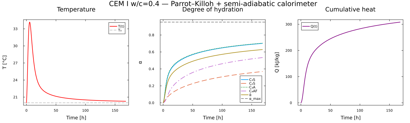
The same two curves on a logarithmic time axis
A hydration curve has to be read on both scales, and each hides what the other shows. Linear time, above, shows where the curve flattens and how much is left to react — the question a 28-day strength depends on. Logarithmic time, below, opens out the first hours: the induction period, the acceleration that follows it, and the peak, all of which happen inside the first decade and are a single vertical rise on a linear axis.
Nothing is recomputed here — the same arrays, a different axis. Two things have to be decided though, and both are about what the axis shows rather than about the chemistry:
t = 0cannot be drawn, sincelog10(0)is-Inf.Nor should the first few steps be. The integrator's first accepted step is at 3.6·10⁻⁴ h — a third of a second — so plotting every positive time spends four of the five decades on an interval where nothing has happened and squeezes the whole of hydration into the right-hand fifth of the panel.
So the axis starts at six minutes — still well inside the induction period, with every α at zero — and carries explicit decade ticks:
t_lo = 0.1                            # h — before this, nothing has happened yet
keep_α = t_h .>= t_lo
keep_Q = t_Q .>= t_lo * 3600
xt = ([0.1, 1.0, 10.0, 100.0], ["0.1", "1", "10", "100"])

p2log = plot(t_h[keep_α],
    [α_C3S[keep_α] α_C2S[keep_α] α_C3A[keep_α] α_C4AF[keep_α] α_mean[keep_α]];
    xscale = :log10, xticks = xt, xlims = (t_lo, 200.0),
    xlabel = "Time [h], log scale", ylabel = "α",
    title = "Degree of hydration", lw = 2, legend = :topleft,
    label = ["C₃S" "C₂S" "C₃A" "C₄AF" "ᾱ"],
    ls = [:solid :dash :dot :dashdot :solid])
hline!(p2log, [α_max]; ls = :dash, color = :black, label = "α_max")

p3log = plot(t_Q[keep_Q] ./ 3600, Q_kJ[keep_Q];
    xscale = :log10, xticks = xt, xlims = (t_lo, 200.0),
    xlabel = "Time [h], log scale", ylabel = "Q [kJ/kg]",
    title = "Cumulative heat", label = "Q(t)", lw = 2, color = :purple,
    legend = :topleft)

plot(p2log, p3log; layout = (1, 2), size = (950, 400),
     left_margin = 8Plots.mm, bottom_margin = 8Plots.mm,
     plot_title = "The same run, logarithmic time")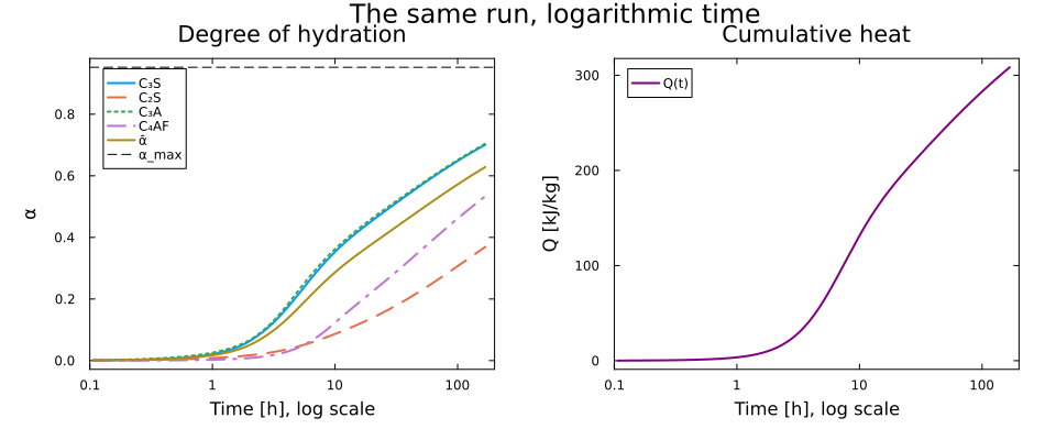
Rather than describe the separation in words, read it off the solution at a few instants:
@printf "%8s %8s %8s %8s %8s %8s\n" "t [h]" "C₃S" "C₂S" "C₃A" "C₄AF" "ᾱ"
for t_target in (1.0, 6.0, 24.0, 168.0)
    i = argmin(abs.(t_h .- t_target))
    @printf("%8.1f %8.3f %8.3f %8.3f %8.3f %8.3f\n",
        t_h[i], α_C3S[i], α_C2S[i], α_C3A[i], α_C4AF[i], α_mean[i])
end
@printf "\nα_max = %.4f (Powers water limit at w/c = %.2f)\n" α_max WC
t [h] C₃S C₂S C₃A C₄AF ᾱ
1.0 0.022 0.009 0.027 0.003 0.018
5.9 0.251 0.054 0.263 0.057 0.200
24.4 0.480 0.155 0.486 0.251 0.403
168.0 0.701 0.369 0.704 0.534 0.628
α_max = 0.9524 (Powers water limit at w/c = 0.40)Two things in that table are worth naming, because both come straight from the parameter sets rather than from the figure:
C₃SandC₃Atrack each other to within a few thousandths at every one of those instants. That is a property of Parrot & Killoh's calibration, not a general fact about cement: the two minerals are given nearly the same diffusion-branch constant,k₂= 0.05 d⁻¹ forC₃Sagainst 0.04 d⁻¹ forC₃A, and it isk₂that governs once the shell has formed.The ranking at seven days is the ranking of
k₂: 0.05, 0.04, 0.015 and 0.006 d⁻¹ forC₃S,C₃A,C₄AFandC₂S, in the same order as the degrees of hydration they reach. Belite's slowness is the well-founded half — the late strength of a Portland cement comes from a mineral that has done about a third of its work after a week.
Each axis answers half the question. The log axis opens out the first hours: the induction period, flat out to about one hour, then C₃S and C₃A accelerating together while C₄AF and C₂S wait several hours more — a spread that is a single vertical rise on a linear axis. The linear axis shows the other half, that none of the curves is anywhere near the ceiling α_max, so this paste still has a great deal of hydration ahead of it when the run stops at seven days.