
Self-desiccation: where Powers' 0.42 comes from
A sealed cement paste stops hydrating before it runs out of cement. Powers' rule of thumb caps the degree of hydration at
and powers_alpha_max supplies it to the rate laws. The coefficient is empirical, and this page takes it apart: it writes the water budget that produces it, fills each term from an independent source — the chemistry from a Gibbs energy minimization, the arrest saturation from a published desorption isotherm — and reports what the two together imply.
Nothing below is fitted to 0.42. The companion script runs the whole calculation outside the documentation.
Read this first: the Kelvin term does not arrest hydration
It is tempting to expect the arrest from thermodynamics — water in a fine pore is held at a reduced activity, so hydrates that consume water become less stable. The magnitude is wrong by two orders of magnitude. At
A real paste stops at 75–80 % relative humidity because transport and nucleation stop. So the humidity belongs in the rate law, through humidity_factor and PoreHumidity, and CapillaryWater is what makes the water activity of the equilibrium state mean the pore water rather than the mole fraction. This page uses the thermodynamics for the water budget and the humidity only as the arrest criterion.
1. The water budget
Take one gram of cement and
Some of it is bound into the hydrate formulae — the
What is left is pore solution, and its volume follows:
And the products occupy less space than the reactants they consumed — the Le Chatelier contraction. In a sealed specimen that deficit cannot be filled from outside, so it becomes empty porosity,
The pore space is therefore liquid plus void, and its degree of saturation is
Now suppose hydration stops when the saturation falls to some value
Two things follow, and the first is a warning about what this page can prove.
Powers' form is structural; only the coefficient is predicted
What is genuinely predicted is
2. The chemistry:
The cement is the one whose isotherm this page uses further down — taking the isotherm from one paper and the clinker from another would compare two materials. (Baroghel-Bouny et al., 1999) give its mineral composition in their Table 2.
using ChemistryLab
using DynamicQuantities
using OptimaSolver
using Printf

# Baroghel-Bouny et al. (1999), Table 2. The balance is free lime and alkalis,
# which this species list does not carry.
compo = ["C3S" => 0.5728, "C2S" => 0.2398, "C3A" => 0.0303,
         "C4AF" => 0.0759, "Gp" => 0.0439, "Cal" => 0.0184]
cmass = sum(last.(compo))
wc    = 0.34                     # their mix CO
M_H2O = 0.0180153                # kg/mol

phases = split("C3S C2S C3A C4AF Gp Anh Cal Portlandite Jennite H2O@ " *
               "ettringite monosulphate12 C3AH6 C3FH6 C4FH13 monocarbonate")
substances = build_species(datapath("cemdata18-thermofun.json"); verbose = false)
cs = ChemicalSystem(
    speciation(substances, phases; aggregate_state = [AS_AQUEOUS]), CEMDATA_PRIMARIES
)
iw = only(cs.idx_solvent)
ic = [findfirst(s -> symbol(s) == sym, cs.species) for (sym, _) in compo]
┌───────────────────────────────────────────────────┐
│ Loading database: data/cemdata18-thermofun.json │
└───────────────────────────────────────────────────┘
┌────────────────────┐
│ Building species │
└────────────────────┘
Progress: 80%|████████████████████████████████████████████████████████████████████████████████████████████████████████████████████████████████▌ | ETA: 0:00:00[K
Progress: 100%|█████████████████████████████████████████████████████████████████████████████████████████████████████████████████████████████████████████████████████████████████| Time: 0:00:00[KAn equilibrium calculation has no notion of a reaction that has not happened, so the degree of hydration is imposed: a fraction
function paste(α)
    mtot = cmass + wc * cmass
    st = ChemicalState(cs)
    for (sym, mfrac) in compo
        set_quantity!(st, sym, α * mfrac / mtot * u"kg")
    end
    set_quantity!(st, "H2O@", wc * cmass / mtot * u"kg")
    V = volume(st)
    set_quantity!(st, "H+", 1e-7u"mol/L" * V.liquid)
    set_quantity!(st, "OH-", 1e-7u"mol/L" * V.liquid)
    return st
end

cement_mass(st) = sum(ustrip(us"kg", st.n[i] * cs.species[i][:M]) for i in ic)

function budget(α)
    fresh = paste(1.0)
    mc    = cement_mass(fresh)
    w_tot = ustrip(us"mol", fresh.n[iw]) * M_H2O
    eq, cert = equilibrate_certified(paste(α))

    n = collect(eq.n)                       # put the unreacted cement back
    for i in ic
        n[i] += (1 - α) * fresh.n[i]
    end
    ϕ = porosity(ChemicalState(cs, n), fresh)

    w_free = ustrip(us"mol", eq.n[iw]) * M_H2O
    V_ref  = ustrip(us"m^3", volume(fresh).total)
    return (; b = (w_tot - w_free) / mc / α,
              s = ϕ.void * V_ref / mc / α * 1e3,      # m³/kg → cm³/g
              w_free = w_free / mc, porosity = ϕ.total, certified = cert.optimal)
end

println(" α      b (g/g)   s (cm³/g)   free water (g/g)   porosity   certified")
for α in (0.55, 0.60, 0.65, 0.70, 0.80)
    r = budget(α)
    @printf("%5.2f  %9.4f  %10.4f  %16.4f  %9.4f   %s\n",
            α, r.b, r.s, r.w_free, r.porosity, r.certified)
end
α b (g/g) s (cm³/g) free water (g/g) porosity certified
┌ Warning: Verbosity toggle: missing_second_order_ad
│ The selected optimization algorithm requires second order derivatives, but `SecondOrder` ADtype was not provided. So a `SecondOrder` with AutoForwardDiff() for both inner and outer will be created, this can be suboptimal and not work in some cases so an explicit `SecondOrder` ADtype is recommended.
└ @ OptimizationBase ~/.julia/packages/OptimizationBase/TvAnm/src/cache.jl:116
0.55 0.3095 0.0640 0.1698 0.3118 true
┌ Warning: Verbosity toggle: missing_second_order_ad
│ The selected optimization algorithm requires second order derivatives, but `SecondOrder` ADtype was not provided. So a `SecondOrder` with AutoForwardDiff() for both inner and outer will be created, this can be suboptimal and not work in some cases so an explicit `SecondOrder` ADtype is recommended.
└ @ OptimizationBase ~/.julia/packages/OptimizationBase/TvAnm/src/cache.jl:116
0.60 0.3095 0.0639 0.1543 0.2931 true
┌ Warning: Verbosity toggle: missing_second_order_ad
│ The selected optimization algorithm requires second order derivatives, but `SecondOrder` ADtype was not provided. So a `SecondOrder` with AutoForwardDiff() for both inner and outer will be created, this can be suboptimal and not work in some cases so an explicit `SecondOrder` ADtype is recommended.
└ @ OptimizationBase ~/.julia/packages/OptimizationBase/TvAnm/src/cache.jl:116
0.65 0.3095 0.0639 0.1389 0.2743 true
┌ Warning: Verbosity toggle: missing_second_order_ad
│ The selected optimization algorithm requires second order derivatives, but `SecondOrder` ADtype was not provided. So a `SecondOrder` with AutoForwardDiff() for both inner and outer will be created, this can be suboptimal and not work in some cases so an explicit `SecondOrder` ADtype is recommended.
└ @ OptimizationBase ~/.julia/packages/OptimizationBase/TvAnm/src/cache.jl:116
0.70 0.3095 0.0639 0.1234 0.2556 true
┌ Warning: Verbosity toggle: missing_second_order_ad
│ The selected optimization algorithm requires second order derivatives, but `SecondOrder` ADtype was not provided. So a `SecondOrder` with AutoForwardDiff() for both inner and outer will be created, this can be suboptimal and not work in some cases so an explicit `SecondOrder` ADtype is recommended.
└ @ OptimizationBase ~/.julia/packages/OptimizationBase/TvAnm/src/cache.jl:116
0.80 0.3095 0.0638 0.0924 0.2182 trueTwo things to read off that table.
Every solve is certified. For a convex problem the KKT conditions are sufficient, so certified = true is a proof that the composition is the Gibbs minimum and not the point an iteration stopped at — see Proving that an answer is the answer.
ref = budget(0.65)
b_model, s_shrink = ref.b, ref.s
@printf("b = %.4f g/g (formula water)     s = %.4f cm³/g (chemical shrinkage)\n",
        b_model, s_shrink)
┌ Warning: Verbosity toggle: missing_second_order_ad
│ The selected optimization algorithm requires second order derivatives, but `SecondOrder` ADtype was not provided. So a `SecondOrder` with AutoForwardDiff() for both inner and outer will be created, this can be suboptimal and not work in some cases so an explicit `SecondOrder` ADtype is recommended.
└ @ OptimizationBase ~/.julia/packages/OptimizationBase/TvAnm/src/cache.jl:116
b = 0.3095 g/g (formula water) s = 0.0639 cm³/g (chemical shrinkage)For scale: a chemical shrinkage of 0.064 cm³ per gram of cement is the value cement chemistry reports for an ordinary Portland cement, and it is here a consequence of the standard molar volumes in the database rather than an input.
3. The measurement:
The retention curve is not chemistry. It says how tightly a particular material holds the water still in it, it is measured, and it is the one thing on this page that cannot come out of a thermodynamic database.
(Baroghel-Bouny et al., 1999) measured water-vapor desorption isotherms on two pastes and two concretes and fitted each with
which is the van Genuchten form written with VanGenuchten as
Their Table 5, with the mixes from their Table 1:
| mix | material | W/C | |||
|---|---|---|---|---|---|
| CO | cement paste | 0.34 | 37.5479 | 2.1684 | 0.46117 |
| CH | paste, 10 % silica fume | 0.19 | 96.2837 | 1.9540 | 0.51177 |
| BO | concrete | 0.48 | 18.6237 | 2.2748 | 0.43960 |
| BH | concrete, 10 % silica fume | 0.26 | 46.9364 | 2.0601 | 0.48541 |
The capillary pressure becomes a water activity through Kelvin, water_activity does:
co    = VanGenuchten(; a = 37.5479e6, m = 1 / 2.1684)   # their mix CO
V_m   = 1.807e-5      # m³/mol, liquid water at 25 °C
T_K   = 298.15
γ_w   = 0.0728        # N/m

a_w(S) = water_activity(co, S; V_m = V_m, T = T_K)

function saturation_at(rh)          # the form is not invertible in closed form
    lo, hi = 1e-4, 1 - 1e-12
    for _ in 1:60
        mid = (lo + hi) / 2
        a_w(mid) > rh ? (hi = mid) : (lo = mid)
    end
    return (lo + hi) / 2
end

println("   RH      S*     p_c (MPa)   Kelvin radius (nm)")
for rh in (0.75, 0.80, 0.85, 0.90, 0.95)
    S = saturation_at(rh)
    @printf("  %4.2f  %6.4f  %10.2f  %18.2f\n", rh, S,
            capillary_pressure(co, S) / 1e6,
            kelvin_radius(rh; γ = γ_w, V_m = V_m, T = T_K) * 1e9)
end
RH S* p_c (MPa) Kelvin radius (nm)
0.75 0.7107 39.47 3.69
0.80 0.7862 30.61 4.76
0.85 0.8619 22.30 6.53
0.90 0.9301 14.45 10.07
0.95 0.9800 7.04 20.69The last column sets the scale: 80 % relative humidity corresponds to a meniscus of radius 4.8 nm. That is the gel-pore scale, which is why the water Powers assigns to gel pores and the water a sealed paste cannot use are the same water.
using Plots

Ss = range(0.40, 0.999; length = 200)
p1 = plot(Ss, a_w.(Ss); xlabel = "degree of saturation S", ylabel = "water activity a_w",
    label = "mix CO, measured fit", linewidth = 2, color = :steelblue,
    title = "Desorption isotherm (Baroghel-Bouny et al. 1999)", legend = :bottomright)
hline!(p1, [0.80]; label = "RH = 0.80", linestyle = :dash, color = :firebrick)
vline!(p1, [saturation_at(0.80)]; label = "S* = $(round(saturation_at(0.80); digits = 4))",
    linestyle = :dash, color = :seagreen)
plot(p1; size = (700, 420), left_margin = 8Plots.mm, bottom_margin = 8Plots.mm)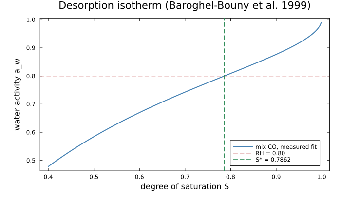
4. Closing the budget
Everything the boxed formula needs is now in hand, each from its own source.
powers_k(b, s, S★) = b + s * S★ / (1 - S★)

S80 = saturation_at(0.80)
@printf("S* = %.4f  so  S*/(1-S*) = %.4f\n\n", S80, S80 / (1 - S80))
@printf("with the model's formula water, b = %.4f:\n", b_model)
@printf("   k = %.4f      α_max(w/c=0.34) = %.4f     (Powers: 0.42 and %.4f)\n",
        powers_k(b_model, s_shrink, S80), wc / powers_k(b_model, s_shrink, S80),
        min(1.0, wc / 0.42))
S* = 0.7862 so S*/(1-S*) = 3.6781
with the model's formula water, b = 0.3095:
k = 0.5445 α_max(w/c=0.34) = 0.6244 (Powers: 0.42 and 0.8095)30 % above Powers. Before calling that a disagreement, look at what
Powers' 0.42 is itself a sum: about 0.23 g/g of non-evaporable water plus about 0.19 g/g of gel water. And his 0.23 is an operational quantity — the water that survives D-drying, over
b_powers = 0.23                     # Powers' non-evaporable water, his own number
@printf("model formula water   %.4f g/g\n", b_model)
@printf("Powers' w_n           %.4f g/g   (defined by D-drying)\n", b_powers)
@printf("difference            %.4f g/g   — interlayer water, counted differently\n",
        b_model - b_powers)
model formula water 0.3095 g/g
Powers' w_n 0.2300 g/g (defined by D-drying)
difference 0.0795 g/g — interlayer water, counted differentlySubstituting Powers' own non-evaporable water, and leaving the chemical shrinkage and the isotherm exactly as measured:
@printf("with Powers' w_n = %.2f:\n", b_powers)
@printf("   k = %.4f      α_max(w/c=0.34) = %.4f     (Powers: 0.42 and %.4f)\n",
        powers_k(b_powers, s_shrink, S80), wc / powers_k(b_powers, s_shrink, S80),
        min(1.0, wc / 0.42))
with Powers' w_n = 0.23:
k = 0.4650 α_max(w/c=0.34) = 0.7311 (Powers: 0.42 and 0.8095)11 % above. The remaining gap is a fifth of a point of saturation, and §6 shows how little that is.
5. The result: inverting Powers
The comparison above runs one way — assume the arrest is at 80 % and see what
function invert_k(b, s, k_target)
    lo, hi = 1e-6, 1 - 1e-12
    for _ in 1:80
        mid = (lo + hi) / 2
        powers_k(b, s, mid) > k_target ? (hi = mid) : (lo = mid)
    end
    return (lo + hi) / 2
end

println("k = 0.42 implies:")
for (label, b) in (("the model's formula water", b_model), ("Powers' own w_n", b_powers))
    S = invert_k(b, s_shrink, 0.42)
    @printf("   b = %.4f (%-26s)   S* = %.4f   RH = %.4f\n", b, label, S, a_w(S))
end
k = 0.42 implies:
b = 0.3095 (the model's formula water ) S* = 0.6337 RH = 0.6956
b = 0.2300 (Powers' own w_n ) S* = 0.7483 RH = 0.7751With Powers' own non-evaporable water, Powers' 0.42 corresponds to a hydration arrest at 77.5 % relative humidity.
That number was not put in anywhere. It came out of a chemical shrinkage computed from a thermodynamic database, a desorption isotherm measured for a drying study, and Powers' own water split — three sources, none of which knows what the others are for. And 75–80 % is the window in which sealed pastes are independently reported to stop hydrating; it is the same window humidity_factor implements as its cut-off.
A corroboration from the same paper's own measurements
(Baroghel-Bouny et al., 1999) also measured the internal relative humidity of their sealed specimens at 28 days, in their Table 3: 97 % for the paste CO (W/C 0.34) and 88.5 % for the paste CH (W/C 0.19); 97 % for the concrete BO (W/C 0.48) and 77.5 % for the concrete BH (W/C 0.26).
Monotone in W/C within each material class, as self-desiccation requires. And the mixes Powers says should have arrested by 28 days — the low-W/C ones — are the ones sitting in the 77.5–88.5 % band that the inversion above points at, while the two mixes with water to spare sit at 97 %. Those specimens are not arrested pastes at equilibrium, so this is corroboration of a range and not a fourth decimal; it is worth stating because the numbers come from the same table as the isotherm.
6. How much of this is the isotherm?
@printf("dk/dS* = %.3f at S* = %.4f\n\n", s_shrink / (1 - S80)^2, S80)
println("   RH      S*        k (model b)   k (Powers w_n)   α_max(0.34)")
for rh in (0.70, 0.75, 0.80, 0.85, 0.90)
    S = saturation_at(rh)
    @printf("  %4.2f  %6.4f  %13.4f  %16.4f  %12.4f\n", rh, S,
            powers_k(b_model, s_shrink, S), powers_k(b_powers, s_shrink, S),
            min(1.0, wc / powers_k(b_powers, s_shrink, S)))
end
dk/dS* = 1.399 at S* = 0.7862
RH S* k (model b) k (Powers w_n) α_max(0.34)
0.70 0.6397 0.4229 0.3435 0.9899
0.75 0.7107 0.4665 0.3870 0.8785
0.80 0.7862 0.5445 0.4650 0.7311
0.85 0.8619 0.7084 0.6290 0.5406
0.90 0.9301 1.1603 1.0808 0.3146rhs = range(0.65, 0.92; length = 120)
ks_m = [powers_k(b_model, s_shrink, saturation_at(r)) for r in rhs]
ks_p = [powers_k(b_powers, s_shrink, saturation_at(r)) for r in rhs]
p2 = plot(rhs, ks_m; xlabel = "assumed arrest humidity", ylabel = "k = (w/c) / α_max",
label = "b = model formula water", linewidth = 2, color = :steelblue,
title = "What the coefficient depends on", legend = :topleft, ylims = (0.25, 1.0))
plot!(p2, rhs, ks_p; label = "b = Powers' w_n = 0.23", linewidth = 2, color = :firebrick)
hline!(p2, [0.42]; label = "Powers 0.42", linestyle = :dash, color = :black)
hline!(p2, [0.36]; label = "Powers 0.36, saturated curing", linestyle = :dot, color = :gray)
plot(p2; size = (700, 420), left_margin = 8Plots.mm, bottom_margin = 8Plots.mm)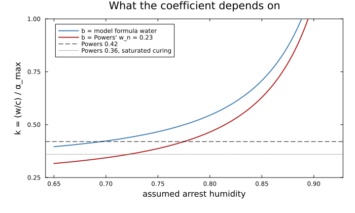
A tenth of a point of saturation moves
7. Two negative controls
Two claims carry the rest of the page: that the arrest criterion belongs in the rate law and not in the Gibbs energy, and that Powers' proportional form is no evidence for his coefficient. Both are testable on the material at hand, so both are measured here rather than asserted.
The thermodynamic route, measured
CapillaryWater imposes a water activity on the equilibrium itself. If self-desiccation arrested hydration thermodynamically, imposing the arrest humidity on a paste with all its cement available would leave some of that cement unreacted. It does not:
fresh = paste(1.0)
ip = findfirst(s -> symbol(s) == "Portlandite", cs.species)
ij = findfirst(s -> symbol(s) == "Jennite", cs.species)

println("  a_w imposed   n(Portlandite)   n(Jennite)   free water (mol)   certified")
for aw in (1.00, 0.90, 0.80, 0.50)
    eq, cert = equilibrate_certified(
        paste(1.0); constraint = CapillaryWater(_ -> aw; reference = fresh)
    )
    @printf("  %11.2f   %14.6f   %10.6f   %16.5f   %s\n", aw,
            ustrip(us"mol", eq.n[ip]), ustrip(us"mol", eq.n[ij]),
            ustrip(us"mol", eq.n[iw]), cert.optimal)
end
a_w imposed n(Portlandite) n(Jennite) free water (mol) certified
┌ Warning: Verbosity toggle: missing_second_order_ad
│ The selected optimization algorithm requires second order derivatives, but `SecondOrder` ADtype was not provided. So a `SecondOrder` with AutoForwardDiff() for both inner and outer will be created, this can be suboptimal and not work in some cases so an explicit `SecondOrder` ADtype is recommended.
└ @ OptimizationBase ~/.julia/packages/OptimizationBase/TvAnm/src/cache.jl:116
1.00 2.659505 2.967346 1.26544 true
┌ Warning: Verbosity toggle: missing_second_order_ad
│ The selected optimization algorithm requires second order derivatives, but `SecondOrder` ADtype was not provided. So a `SecondOrder` with AutoForwardDiff() for both inner and outer will be created, this can be suboptimal and not work in some cases so an explicit `SecondOrder` ADtype is recommended.
└ @ OptimizationBase ~/.julia/packages/OptimizationBase/TvAnm/src/cache.jl:116
0.90 2.659505 2.967345 1.26544 true
┌ Warning: Verbosity toggle: missing_second_order_ad
│ The selected optimization algorithm requires second order derivatives, but `SecondOrder` ADtype was not provided. So a `SecondOrder` with AutoForwardDiff() for both inner and outer will be created, this can be suboptimal and not work in some cases so an explicit `SecondOrder` ADtype is recommended.
└ @ OptimizationBase ~/.julia/packages/OptimizationBase/TvAnm/src/cache.jl:116
0.80 2.659505 2.967345 1.26545 true
┌ Warning: Verbosity toggle: missing_second_order_ad
│ The selected optimization algorithm requires second order derivatives, but `SecondOrder` ADtype was not provided. So a `SecondOrder` with AutoForwardDiff() for both inner and outer will be created, this can be suboptimal and not work in some cases so an explicit `SecondOrder` ADtype is recommended.
└ @ OptimizationBase ~/.julia/packages/OptimizationBase/TvAnm/src/cache.jl:116
┌ Warning: Verbosity toggle: missing_second_order_ad
│ The selected optimization algorithm requires second order derivatives, but `SecondOrder` ADtype was not provided. So a `SecondOrder` with AutoForwardDiff() for both inner and outer will be created, this can be suboptimal and not work in some cases so an explicit `SecondOrder` ADtype is recommended.
└ @ OptimizationBase ~/.julia/packages/OptimizationBase/TvAnm/src/cache.jl:116
┌ Warning: Verbosity toggle: missing_second_order_ad
│ The selected optimization algorithm requires second order derivatives, but `SecondOrder` ADtype was not provided. So a `SecondOrder` with AutoForwardDiff() for both inner and outer will be created, this can be suboptimal and not work in some cases so an explicit `SecondOrder` ADtype is recommended.
└ @ OptimizationBase ~/.julia/packages/OptimizationBase/TvAnm/src/cache.jl:116
┌ Warning: Verbosity toggle: missing_second_order_ad
│ The selected optimization algorithm requires second order derivatives, but `SecondOrder` ADtype was not provided. So a `SecondOrder` with AutoForwardDiff() for both inner and outer will be created, this can be suboptimal and not work in some cases so an explicit `SecondOrder` ADtype is recommended.
└ @ OptimizationBase ~/.julia/packages/OptimizationBase/TvAnm/src/cache.jl:116
┌ Warning: Verbosity toggle: missing_second_order_ad
│ The selected optimization algorithm requires second order derivatives, but `SecondOrder` ADtype was not provided. So a `SecondOrder` with AutoForwardDiff() for both inner and outer will be created, this can be suboptimal and not work in some cases so an explicit `SecondOrder` ADtype is recommended.
└ @ OptimizationBase ~/.julia/packages/OptimizationBase/TvAnm/src/cache.jl:116
┌ Warning: Verbosity toggle: missing_second_order_ad
│ The selected optimization algorithm requires second order derivatives, but `SecondOrder` ADtype was not provided. So a `SecondOrder` with AutoForwardDiff() for both inner and outer will be created, this can be suboptimal and not work in some cases so an explicit `SecondOrder` ADtype is recommended.
└ @ OptimizationBase ~/.julia/packages/OptimizationBase/TvAnm/src/cache.jl:116
┌ Warning: Verbosity toggle: missing_second_order_ad
│ The selected optimization algorithm requires second order derivatives, but `SecondOrder` ADtype was not provided. So a `SecondOrder` with AutoForwardDiff() for both inner and outer will be created, this can be suboptimal and not work in some cases so an explicit `SecondOrder` ADtype is recommended.
└ @ OptimizationBase ~/.julia/packages/OptimizationBase/TvAnm/src/cache.jl:116
┌ Warning: Verbosity toggle: missing_second_order_ad
│ The selected optimization algorithm requires second order derivatives, but `SecondOrder` ADtype was not provided. So a `SecondOrder` with AutoForwardDiff() for both inner and outer will be created, this can be suboptimal and not work in some cases so an explicit `SecondOrder` ADtype is recommended.
└ @ OptimizationBase ~/.julia/packages/OptimizationBase/TvAnm/src/cache.jl:116
┌ Warning: Verbosity toggle: missing_second_order_ad
│ The selected optimization algorithm requires second order derivatives, but `SecondOrder` ADtype was not provided. So a `SecondOrder` with AutoForwardDiff() for both inner and outer will be created, this can be suboptimal and not work in some cases so an explicit `SecondOrder` ADtype is recommended.
└ @ OptimizationBase ~/.julia/packages/OptimizationBase/TvAnm/src/cache.jl:116
┌ Warning: Verbosity toggle: missing_second_order_ad
│ The selected optimization algorithm requires second order derivatives, but `SecondOrder` ADtype was not provided. So a `SecondOrder` with AutoForwardDiff() for both inner and outer will be created, this can be suboptimal and not work in some cases so an explicit `SecondOrder` ADtype is recommended.
└ @ OptimizationBase ~/.julia/packages/OptimizationBase/TvAnm/src/cache.jl:116
┌ Warning: Verbosity toggle: missing_second_order_ad
│ The selected optimization algorithm requires second order derivatives, but `SecondOrder` ADtype was not provided. So a `SecondOrder` with AutoForwardDiff() for both inner and outer will be created, this can be suboptimal and not work in some cases so an explicit `SecondOrder` ADtype is recommended.
└ @ OptimizationBase ~/.julia/packages/OptimizationBase/TvAnm/src/cache.jl:116
┌ Warning: Verbosity toggle: missing_second_order_ad
│ The selected optimization algorithm requires second order derivatives, but `SecondOrder` ADtype was not provided. So a `SecondOrder` with AutoForwardDiff() for both inner and outer will be created, this can be suboptimal and not work in some cases so an explicit `SecondOrder` ADtype is recommended.
└ @ OptimizationBase ~/.julia/packages/OptimizationBase/TvAnm/src/cache.jl:116
┌ Warning: Verbosity toggle: missing_second_order_ad
│ The selected optimization algorithm requires second order derivatives, but `SecondOrder` ADtype was not provided. So a `SecondOrder` with AutoForwardDiff() for both inner and outer will be created, this can be suboptimal and not work in some cases so an explicit `SecondOrder` ADtype is recommended.
└ @ OptimizationBase ~/.julia/packages/OptimizationBase/TvAnm/src/cache.jl:116
┌ Warning: Verbosity toggle: missing_second_order_ad
│ The selected optimization algorithm requires second order derivatives, but `SecondOrder` ADtype was not provided. So a `SecondOrder` with AutoForwardDiff() for both inner and outer will be created, this can be suboptimal and not work in some cases so an explicit `SecondOrder` ADtype is recommended.
└ @ OptimizationBase ~/.julia/packages/OptimizationBase/TvAnm/src/cache.jl:116
┌ Warning: Verbosity toggle: missing_second_order_ad
│ The selected optimization algorithm requires second order derivatives, but `SecondOrder` ADtype was not provided. So a `SecondOrder` with AutoForwardDiff() for both inner and outer will be created, this can be suboptimal and not work in some cases so an explicit `SecondOrder` ADtype is recommended.
└ @ OptimizationBase ~/.julia/packages/OptimizationBase/TvAnm/src/cache.jl:116
┌ Warning: no route produced a certifiable equilibrium: stationarity 9.693212043424294e-15, element balance 8.633094239485217e-13, worst supersaturation 1.7243195661912978. Automatic initial approximation: the continuation improved the KKT error from 1.7243195662313155 to 1.7243195662076687 without certifying; returning the answer with the smallest KKT error — audit it with `optimality_certificate`
└ @ ChemistryLab ~/work/ChemistryLab.jl/ChemistryLab.jl/src/equilibrium/certified.jl:845
0.50 2.659512 2.967344 1.26575 falseFrom saturation down to the arrest humidity the assemblage is identical to six digits — the imposed shift moves the answer by less than the printing precision — and each of those answers is certified. The last row is there to show the other half of that: further down, no route certifies, the warning above the table is equilibrate_certified saying so, and the answer it returns is a KKT candidate rather than a proof. The arithmetic in the opening admonition says why nothing is expected to happen in that range anyway.
So a Gibbs minimization under CapillaryWater arrests where it ran out of water stoichiometrically, not where Powers says. What the constraint is good for is what §3–§5 use it for: making the water activity of a state mean the water in the pores rather than a mole fraction, and handing that humidity to a rate law through PoreHumidity.
The proportional form, measured
§1 argued that
bh = VanGenuchten(; a = 46.9364e6, m = 1 / 2.0601)   # their mix BH

function saturation_of(law, rh)
    lo, hi = 1e-4, 1 - 1e-12
    for _ in 1:60
        mid = (lo + hi) / 2
        water_activity(law, mid; V_m = V_m, T = T_K) > rh ? (hi = mid) : (lo = mid)
    end
    return (lo + hi) / 2
end

for (name, law) in (("CO", co), ("BH", bh))
    S = saturation_of(law, 0.80)
    k = powers_k(b_model, s_shrink, S)
    @printf("\ncurve %s:  S* = %.4f   k = %.4f\n", name, S, k)
    for w in (0.25, 0.30, 0.35, 0.40)
        @printf("   w/c %.2f  →  α_max = %.6f   α_max/(w/c) = %.6f\n", w, w / k, 1 / k)
    end
end
curve CO:  S* = 0.7862   k = 0.5445
   w/c 0.25  →  α_max = 0.459134   α_max/(w/c) = 1.836536
   w/c 0.30  →  α_max = 0.550961   α_max/(w/c) = 1.836536
   w/c 0.35  →  α_max = 0.642788   α_max/(w/c) = 1.836536
   w/c 0.40  →  α_max = 0.734615   α_max/(w/c) = 1.836536

curve BH:  S* = 0.8390   k = 0.6424
   w/c 0.25  →  α_max = 0.389172   α_max/(w/c) = 1.556689
   w/c 0.30  →  α_max = 0.467007   α_max/(w/c) = 1.556689
   w/c 0.35  →  α_max = 0.544841   α_max/(w/c) = 1.556689
   w/c 0.40  →  α_max = 0.622676   α_max/(w/c) = 1.556689
The last column is the same number at every
Neither curve gives 0.42 at RH 0.80 with this system's formula water. Recovering Powers' coefficient takes his own water split as well, and §5 does that explicitly and says so.
8. What went in, and what came out
| input | value | source | is that source about Powers? |
|---|---|---|---|
| clinker composition | Table 2 | (Baroghel-Bouny et al., 1999) | no |
| thermodynamic data | Cemdata18 | (Lothenbach et al., 2019) | no |
| 0.3095 g/g, 0.0639 cm³/g | computed here, certified | no | |
| retention curve | (Baroghel-Bouny et al., 1999) Table 5 | no | |
| 0.0728 N/m, 1.807e-5 m³/mol, 298.15 K | water at 25 °C | no | |
| Powers' own split of his 0.42 | (Powers, 1948) | yes |
output: the arrest humidity, 77.5 %.
Only the last row knows about Powers, and it contributes his decomposition, not his coefficient. Nothing on this page was adjusted to improve the agreement, and the one number that could have been — the retention curve — was fitted by its authors to a drying experiment two decades before this calculation existed.
9. Assumptions, and where each one bites
The degree of hydration is imposed, not predicted. §2's construction reacts a fraction of the cement and leaves the rest inert. What this page computes is the
at which the arrest criterion is met, not a trajectory in time. For that, hand PoreHumiditytoparrot_killoh_avramias itshumidityand integrate.One retention curve for an evolving pore structure. The measured isotherm belongs to a mature paste; the page applies it at every
. The pore structure of a young paste is coarser, so its true is higher and the arrest earlier. The published fit excludes the humidity range this page works in. The authors state that "the experimental data corresponding to the lowest capillary pressures (corresponding to the highest RH) have not been accounted [for] due to their weak reliability". Above about 90 % RH the curve used here is extrapolation into a region its authors declined to fit — which is exactly where an unarrested paste sits, and a reason the corroboration in §5 is stated as a range.
The saturations are normalized differently. The paper's
is relative to its measured total porosity, 30.3 % for mix CO; this model gives 27.4 % at , and by §6 worth a few hundredths of . The C-S-H model matters as much as the isotherm.
one for one. Measured on this system: Jennitegives= 0.3095 g/g and the CSHQsolid solution gives 0.3684, so it moves away from Powers, not toward him. Neither is wrong; they draw the formula-water line in different places.No alkalis. This species list carries none, so the pore solution's osmotic depression of
is absent. At 0.1–0.5 mol/kg it is worth one to two points of relative humidity, in the same direction as the capillary term. Ideal molar volumes, and a closed species list — the standing assumptions of every equilibrium page here.
10. Reproducing this
julia --project=scripts scripts/self_desiccation_powers.jlEvery block above is executed when this page is built, so the numbers printed are whatever the code produced. The script computes the same quantities outside Documenter and prints the intermediate ones this page summarizes.
See also: CapillaryWater, PoreHumidity, WaterRetention, powers_alpha_max, and the w/c example, which shows what a Gibbs minimization does without an arrest criterion.