Solid solution models, in numbers

Solid solutions derives the three mixing models and says what each parameter means. This page evaluates them: what an end-member's activity actually is, where a regular solution stops being one phase, and a check that the two non-ideal models agree where they must.

Nothing is solved here either — these are the mixing expressions on their own, which is the cheapest way to see what a parameter does before putting it in a SolidSolutionPhase.

julia

using ChemistryLab
using Printf

RT25 = 8.31446261815324 * 298.15        # J/mol at 25 °C

1. Where a regular solution stops being one phase

A symmetric binary has , and it unmixes wherever that is concave. The second derivative at equal fractions is , so the critical point sits at — about 5 kJ/mol at 25 °C:

julia

d2G(x, w) = 1 / x + 1 / (1 - x) - 2w          # w = W/RT
verdict(v) = abs(v) < 1.0e-12 ? "critical point" : v > 0 ? "one phase" : "unmixes"
println("  W/RT    W (kJ/mol)    ∂²(G/RT)/∂x² at x = 0.5    verdict")
for w in (0.0, 1.0, 1.9, 2.0, 2.1, 3.0)
    @printf("%6.2f   %10.2f   %22.3f    %s\n",
            w, w * RT25 / 1000, d2G(0.5, w), verdict(d2G(0.5, w)))
end

  W/RT    W (kJ/mol)    ∂²(G/RT)/∂x² at x = 0.5    verdict
  0.00         0.00                    4.000    one phase
  1.00         2.48                    2.000    one phase
  1.90         4.71                    0.200    one phase
  2.00         4.96                    0.000    critical point
  2.10         5.21                   -0.200    unmixes
  3.00         7.44                   -2.000    unmixes

This has to be checked before a parameter goes into a model, because nothing in the equilibrium solver detects it: because a solid solution is entered as one phase and the activity expression keeps returning numbers on the wrong side of the threshold. Those numbers describe a metastable single phase.

Seen as the Gibbs energy of mixing itself, the threshold is the moment the curve stops being convex:

julia

using Plots

xs = range(0.001, 0.999; length = 300)
Gmix(x, w) = x * log(x) + (1 - x) * log(1 - x) + w * x * (1 - x)

p1 = plot(; xlabel = "mole fraction x₁", ylabel = "G_mix / RT",
    title = "Mixing free energy across the critical point", legend = :bottom)
for (w, col, st) in ((0.0, :steelblue, :solid), (1.0, :seagreen, :solid),
                     (2.0, :black, :dash), (2.5, :darkorange, :solid),
                     (3.0, :firebrick, :solid))
    plot!(p1, xs, [Gmix(x, w) for x in xs];
        label = "W/RT = $(w)" * (w == 2.0 ? "  (critical)" : ""),
        linewidth = 2, color = col, linestyle = st)
end
plot(p1; size = (720, 430), left_margin = 10Plots.mm, bottom_margin = 8Plots.mm)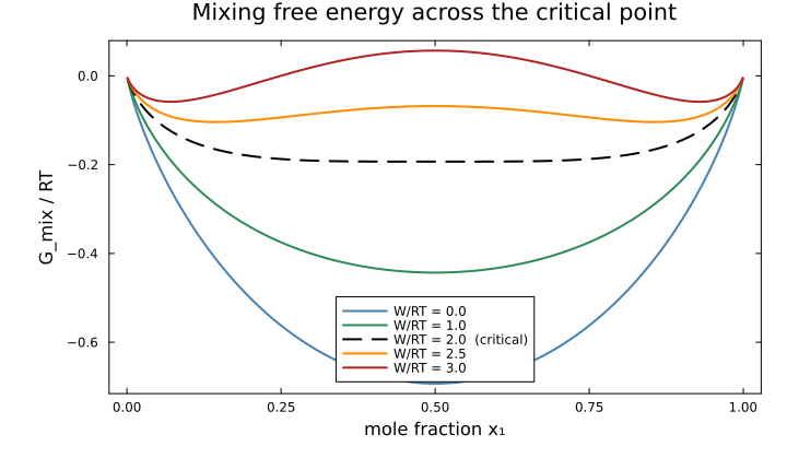

Below the critical value the curve is convex everywhere and a single phase is stable at every composition. Above it a hump appears in the middle: a mixture there lowers its energy by separating into two phases, one at each side of the hump. At W/RT = 2 exactly the curve is flat to second order at x = 0.5, which is what the table above measures.

2. Redlich-Kister reduces to a regular solution, as it must

is the symmetric term of the Redlich-Kister expansion, so it is exactly a regular solution's , and setting the asymmetric terms to zero must reproduce the other model. Two independently written methods, one identity:

julia

W = 12_000.0        # J/mol
T = 298.15
x = [0.3, 0.7]

reg = RegularSolutionModel([0.0 W; W 0.0])
rk = RedlichKisterModel(a0 = W, a1 = 0.0, a2 = 0.0)

for k in 1:2
    lr = ChemistryLab._excess_ln_gamma(reg, k, x, T)
    lk = ChemistryLab._excess_ln_gamma(rk, k, x, T)
    @printf("end-member %d:  regular ln γ = %+.10f   Redlich-Kister ln γ = %+.10f   Δ = %.2e\n",
            k, lr, lk, abs(lr - lk))
end

end-member 1:  regular ln γ = +2.3719652781   Redlich-Kister ln γ = +2.3719652781   Δ = 0.00e+00
end-member 2:  regular ln γ = +0.4356670919   Redlich-Kister ln γ = +0.4356670919   Δ = 5.55e-17

This corresponds to , past the critical value of 2 from §1. The identity is algebraic and holds regardless of stability, but the composition it is evaluated at is not one a homogeneous phase would occupy.

3. What the models do to an activity

kJ/mol below, which is — inside the stable range on purpose, so the numbers describe a phase that stays homogeneous:

julia

models = ["ideal" => IdealSolidSolutionModel(),
          "regular W>0" => RegularSolutionModel([0.0 4000.0; 4000.0 0.0]),
          "regular W<0" => RegularSolutionModel([0.0 -4000.0; -4000.0 0.0])]

@printf("W/RT = %+.2f, so §1 says one phase everywhere\n\n", 4000.0 / RT25)
println("            a₁ = x₁ γ₁")
println("   x₁      ideal    W>0      W<0")
for x1 in (0.01, 0.1, 0.3, 0.5, 0.7, 0.9)
    xs = [x1, 1 - x1]
    a = [x1 * exp(ChemistryLab._excess_ln_gamma(mod, 1, xs, 298.15)) for (_, mod) in models]
    @printf("%6.2f   %7.4f  %7.4f  %7.4f\n", x1, a...)
end

W/RT = +1.61, so §1 says one phase everywhere

            a₁ = x₁ γ₁
   x₁      ideal    W>0      W<0
┌ Warning: Assignment to `xs` in soft scope is ambiguous because a global variable by the same name exists: `xs` will be treated as a new local. Disambiguate by using `local xs` to suppress this warning or `global xs` to assign to the existing global variable.
└ @ solid_solution_models.md:110
  0.01    0.0100   0.0486   0.0021
  0.10    0.1000   0.3695   0.0271
  0.30    0.3000   0.6615   0.1361
  0.50    0.5000   0.7484   0.3340
  0.70    0.7000   0.8094   0.6054
  0.90    0.9000   0.9146   0.8856

Two consequences. A positive pushes the activity of a dilute end-member above its mole fraction — the host is rejecting it — while a negative pulls it below, the host stabilizing it. And at all three converge, because as the phase becomes pure: the standard state of an end-member is the pure end-member, and the models agree there by construction.

The ideal column is the relevant one for cement. An end-member at has , so its saturation index is shifted three decades below the pure phase — a trace component is stabilized simply by being diluted in a host, which is how a solid solution takes up an ion that would never precipitate on its own.

julia

p2 = plot(; xlabel = "mole fraction x₁", ylabel = "activity a₁",
    title = "An end-member's activity, and what W does to it", legend = :topleft)
plot!(p2, xs, collect(xs); label = "ideal (a = x)", linewidth = 2, color = :black,
    linestyle = :dot)
for (W, col) in ((4000.0, :firebrick), (-4000.0, :steelblue))
    mod = RegularSolutionModel([0.0 W; W 0.0])
    plot!(p2, xs, [x * exp(ChemistryLab._excess_ln_gamma(mod, 1, [x, 1 - x], 298.15))
                   for x in xs];
        label = "W = $(round(Int, W / 1000)) kJ/mol", linewidth = 2, color = col)
end
plot(p2; size = (720, 430), left_margin = 8Plots.mm, bottom_margin = 8Plots.mm)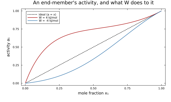

The three curves meet at x₁ = 1, where the standard state is, and separate most at the dilute end — which is exactly where a solid solution decides whether it will take up a trace component.

See also: Solid solutions for the derivations, and What the choice of activity model costs for the same exercise on the aqueous side.

Solid solution models, in numbers ​

1. Where a regular solution stops being one phase ​

2. Redlich-Kister reduces to a regular solution, as it must ​

3. What the models do to an activity ​

Solid solution models, in numbers

1. Where a regular solution stops being one phase

2. Redlich-Kister reduces to a regular solution, as it must

3. What the models do to an activity