Carbonation of a Cement Paste

Carbonation is the principal durability threat to reinforced concrete. Atmospheric CO₂ diffuses into the concrete cover, dissolves into the pore water, and reacts with the alkaline hydration products — above all portlandite Ca(OH)₂ and calcium silicate hydrates (CSH) — to precipitate calcium carbonate (calcite):

This consumption of alkalinity drives the pore-solution pH from ≈ 12.5–13 down to ≈ 8–9, below the passivation threshold of the steel reinforcement (~9.5). The depth at which pH drops below this threshold is the carbonation front.

This example simulates the progressive carbonation of a reference hydrated cement paste by scanning the CO₂ intake from zero to 2.5× the stoichiometric portlandite capacity. It tracks the pH of the pore solution, the depletion of portlandite and CSH, and the accumulation of calcite.

System setup

The CEMDATA18-merged database is used here because it contains both the cement hydration products and the carbonate mineral phases (calcite Cal, monocarbonate, hemicarbonate) within a single consistent dataset.

The species list covers the full mineralogy of a hydrating and carbonating Portland cement paste: clinker phases, classic hydration products, and the three principal carbonation products.

Group	Symbols	Role
Clinker	`C3S C2S C3A C4AF Gp`	Initial anhydrous phases
Hydration products	`Portlandite Jennite ettringite monosulphate12 C3AH6`	Formed during hydration
Carbonation products	`Cal monocarbonate hemicarbonate`	Formed on CO₂ uptake
CO₂ input	`CO2@`	Dissolved CO₂ entering the pore solution

julia

input_species = split("""C3S C2S C3A C4AF Gp
                         Portlandite Jennite ettringite monosulphate12 C3AH6
                         Cal monocarbonate hemicarbonate
                         CO2@""")

species = speciation(
    substances, input_species;
    aggregate_state   = [AS_AQUEOUS],
    exclude_species   = split("H2@ O2@ H2S@ HS- thaumasite Arg"),
    include_species   = input_species,
)

cs = ChemicalSystem(species, CEMDATA_PRIMARIES)

The chemical system in full — species, phases and the conservation matrix

julia

cs

58-element ChemicalSystem{Species, AbstractReaction, StoichMatrix{Real, Symbol, Vector{Symbol}, Matrix{Real}, Species}, StoichMatrix{Real, Species, Vector{Species}, Matrix{Real}, Species}, Nothing}:
 H2O@ {H2O  l} [H2O@ ◆ H₂O@]
 CaSiO3@ {CaSiO3  aq } [CaSiO3@ ◆ CaSiO₃@]
 SiO3-2 {SiO3-2  aq } [SiO3-2 ◆ SiO₃²⁻]
 AlSiO5-3 {AlSiO5-3  aq } [AlSiO5-3 ◆ AlSiO₅³⁻]
 Si4O10-4 {Si4O10-4  aq } [Si4O10-4 ◆ Si₄O₁₀⁴⁻]
 SiO2@ {SiO2  aq ( + 2 H2O = Si(OH)4  aq )} [SiO2@ ◆ SiO₂@]
 Al(SO4)2- {Al(SO4)2-} [Al(SO4)2- ◆ Al(SO₄)₂⁻]
 Fe(SO4)@ {FeSO4  aq} [Fe(SO4)@ ◆ Fe(SO₄)@]
 Fe(SO4)+ {FeSO4+} [Fe|3|(SO4)+ ◆ Fe(SO₄)⁺]
 Fe(SO4)2- {Fe(SO4)2-} [Fe|3|(SO4)2- ◆ Fe(SO₄)₂⁻]
 Fe(CO3)@ {FeCO3  aq} [FeCO3@ ◆ FeCO₃@]
 Al(SO4)+ {AlSO4+} [Al(SO4)+ ◆ Al(SO₄)⁺]
 Fe(HCO3)+ {FeHCO3+} [FeHCO3+ ◆ FeHCO₃⁺]
 Fe(HSO4)+2 {FeHSO4+2} [Fe|3|HSO4+2 ◆ FeHSO₄²⁺]
 Fe(HSO4)+ {FeHSO4+} [FeHSO4+ ◆ FeHSO₄⁺]
 Al+3 {Al+3} [Al+3 ◆ Al³⁺]
 Ca+2 {Ca+2} [Ca+2 ◆ Ca²⁺]
 Fe+2 {Fe+2} [Fe+2 ◆ Fe²⁺]
 H+ {H+} [H+ ◆ H⁺]
 HCO3- {HCO3-} [HCO3- ◆ HCO₃⁻]
 SO4-2 {SO4-2} [S|6|O4-2 ◆ SO₄²⁻]
 AlO2- {AlO2-  ( + 2 H2O = Al(OH)4- )} [AlO2- ◆ AlO₂⁻]
 CO3-2 {CO3-2} [CO3-2 ◆ CO₃²⁻]
 FeO2- {FeO2- ( + 2 H2O = Fe(OH)4- )} [Fe|3|O2- ◆ FeO₂⁻]
 AlOH+2 {AlOH+2} [Al(OH)+2 ◆ Al(OH)²⁺]
 AlO+ {AlO+  ( + H2O = Al(OH)2+ )} [AlO+ ◆ AlO⁺]
 AlO2H@ {AlO2H  aq ( + 2H2O = Al(OH)3  aq )} [AlO2H@ ◆ AlO₂H@]
 CaOH+ {CaOH+} [Ca(OH)+ ◆ Ca(OH)⁺]
 FeOH+2 {FeOH+2} [Fe|3|(OH)+2 ◆ Fe(OH)²⁺]
 FeO+ {FeO+ ( + H2O = Fe(OH)2+ )} [Fe|3|O+ ◆ FeO⁺]
 FeO2H@ {FeO2H  aq  ( + H2O = Fe(OH)3  aq)} [Fe|3|O2H@ ◆ FeO₂H@]
 FeOH+ {FeOH+} [FeOH+ ◆ FeOH⁺]
 HSO3- {HSO3-} [HS|4|O3- ◆ HSO₃⁻]
 HSO4- {HSO4-} [HS|6|O4- ◆ HSO₄⁻]
 OH- {OH-} [OH- ◆ OH⁻]
 S2O3-2 {S2O3-2} [S|2|2O3-2 ◆ S₂O₃²⁻]
 SO3-2 {SO3-2} [S|4|O3-2 ◆ SO₃²⁻]
 Fe+3 {Fe+3} [Fe|3|+3 ◆ Fe³⁺]
 CH4@ {CH4  aq} [C|-4|H4@ ◆ CH₄@]
 Ca(HCO3)+ {CaHCO3+} [Ca(HCO3)+ ◆ Ca(HCO₃)⁺]
 Ca(HSiO3)+ {CaHSiO3+  ( + H2O = CaSiO(OH)3+ )} [Ca(HSiO3)+ ◆ Ca(HSiO₃)⁺]
 CO2@ {CO2  aq} [CO2@ ◆ CO₂@]
 Ca(CO3)@ {CaCO3  aq} [CaCO3@ ◆ CaCO₃@]
 Ca(SO4)@ {CaSO4  aq} [CaSO4@ ◆ CaSO₄@]
 HSiO3- {HSiO3-  ( + H2O = SiO(OH)3- )} [HSiO3- ◆ HSiO₃⁻]
 monosulphate12 {Monosulphate12} [Ca4Al2SO10(H2O)12 ◆ Ca₄Al₂SO₁₀(H₂O)₁₂]
 Jennite {Jennite   10/6 end-member of  id CSH SS (norm per 1 Si)  } [(SiO2)1(CaO)1.666667(H2O)2.1 ◆ (SiO₂)₁(CaO)₅//₃(H₂O)₂.₁]
 monocarbonate {Monocarbonate} [Ca4Al2CO9(H2O)11 ◆ Ca₄Al₂CO₉(H₂O)₁₁]
 C3S {C3S} [(CaO)3SiO2 ◆ (CaO)₃SiO₂]
 C2S {C2S-beta} [(CaO)2SiO2 ◆ (CaO)₂SiO₂]
 C3A {C3A (3CaO_Al2O3)} [(CaO)3Al2O3 ◆ (CaO)₃Al₂O₃]
 C4AF {C4AF} [(CaO)4(Al2O3)(Fe|3|2O3) ◆ (CaO)₄(Al₂O₃)(Fe₂O₃)]
 ettringite {Ettringite with 32 H2O} [((H2O)2)Ca6Al2(SO4)3(OH)12(H2O)24 ◆ ((H₂O)₂)Ca₆Al₂(SO₄)₃(OH)₁₂(H₂O)₂₄]
 C3AH6 {C3AH6} [Ca3Al2O6(H2O)6 ◆ Ca₃Al₂O₆(H₂O)₆]
 hemicarbonate {Hemicarbonate} [(CaO)3Al2O3(CaCO3)0.5(CaO2H2)0.5(H2O)11.5 ◆ (CaO)₃Al₂O₃(CaCO₃)½(CaO₂H₂)½(H₂O)₂₃//₂]
 Portlandite {Portlandite} [Ca(OH)2 ◆ Ca(OH)₂]
 Gp {Gypsum} [CaSO4(H2O)2 ◆ CaSO₄(H₂O)₂]
 Cal {Calcite} [CaCO3 ◆ CaCO₃]

Why cemdata18-merged?

Not for calcite: Cal is present in cemdata18-thermofun.json too, and an earlier version of this note said otherwise. Nor for species at all — both files describe the same 228 substances. What the PHREEQC .dat file brings is the reactions, 148 against 7, and with them the phase-volume data that makes volumes and porosity available on one consistent dataset.

Building the equilibrium solver

A single solver is compiled once and reused for all calculations.

julia

using Optimization, OptimizationIpopt

opt = IpoptOptimizer(
    acceptable_tol        = 1e-10,
    dual_inf_tol          = 1e-10,
    acceptable_iter       = 100,
    constr_viol_tol       = 1e-10,
    warm_start_init_point = "no",
)

solver = EquilibriumSolver(
    cs,
    DiluteSolutionModel(),
    opt;
    variable_space = Val(:linear),
    abstol  = 1e-8,
    reltol  = 1e-8,
)

sp_idx = Dict(symbol(s) => i for (i, s) in enumerate(cs.species))

Dict{String, Int64} with 58 entries:
  "SiO2@"          => 6
  "AlO2-"          => 22
  "Fe(HCO3)+"      => 13
  "Fe(CO3)@"       => 11
  "Fe(SO4)@"       => 8
  "FeO2-"          => 24
  "HSiO3-"         => 45
  "C3AH6"          => 54
  "S2O3-2"         => 36
  "FeO+"           => 30
  "Fe+2"           => 18
  "FeOH+2"         => 29
  "SO4-2"          => 21
  "Jennite"        => 47
  "Si4O10-4"       => 5
  "Al(SO4)2-"      => 7
  "monocarbonate"  => 48
  "CO2@"           => 42
  "Fe(SO4)+"       => 9
  "C3S"            => 49
  "CaSiO3@"        => 2
  "CO3-2"          => 23
  "Al+3"           => 16
  "Cal"            => 58
  "Fe(HSO4)+2"     => 14
  "Ca+2"           => 17
  "HSO4-"          => 34
  "HSO3-"          => 33
  "OH-"            => 35
  "AlOH+2"         => 25
  "H2O@"           => 1
  "Ca(HCO3)+"      => 40
  "C3A"            => 51
  "Al(SO4)+"       => 12
  "FeOH+"          => 32
  "C4AF"           => 52
  "hemicarbonate"  => 55
  "FeO2H@"         => 31
  "SO3-2"          => 37
  "SiO3-2"         => 3
  "CaOH+"          => 28
  "AlSiO5-3"       => 4
  "HCO3-"          => 20
  "H+"             => 19
  "Fe+3"           => 38
  "CH4@"           => 39
  "Fe(SO4)2-"      => 10
  "monosulphate12" => 46
  "ettringite"     => 53
  "Ca(CO3)@"       => 43
  "Gp"             => 57
  "AlO2H@"         => 27
  "Portlandite"    => 56
  "Ca(HSiO3)+"     => 41
  "Ca(SO4)@"       => 44
  "AlO+"           => 26
  "C2S"            => 50
  "Fe(HSO4)+"      => 15

Step 1 — Reference hydrated paste (no CO₂)

Before scanning the carbonation, the reference state of the fully hydrated paste is established by solving the equilibrium without any CO₂ input. This gives the initial portlandite inventory, which is used to normalize the CO₂ axis.

julia

compo = ["C3S" => 0.678, "C2S" => 0.166, "C3A" => 0.040, "C4AF" => 0.072, "Gp" => 0.028]
c     = sum(last.(compo))   # ≈ 0.984
wc    = 0.40
w     = wc * c
mtot  = c + w

state0 = ChemicalState(cs)
for (sym, mfrac) in compo
    set_quantity!(state0, sym, mfrac / mtot * u"kg")
end
set_quantity!(state0, "H2O@", w / mtot * u"kg")

V0 = volume(state0)
set_quantity!(state0, "H+",  1e-7u"mol/L" * V0.liquid)
set_quantity!(state0, "OH-", 1e-7u"mol/L" * V0.liquid)

ref = solve(solver, state0)

n_port0 = ustrip(ref.n[sp_idx["Portlandite"]])
n_ett0  = ustrip(ref.n[sp_idx["ettringite"]])
n_jen0  = ustrip(ref.n[sp_idx["Jennite"]])

println("Reference state (w/c = 0.40, no CO₂):")
println("  pH          = ", round(pH(ref),         digits = 2))
println("  Portlandite = ", round(n_port0,          digits = 3), " mol/kg")
println("  Ettringite  = ", round(n_ett0,           digits = 3), " mol/kg")
println("  Jennite     = ", round(n_jen0,           digits = 3), " mol/kg")
println("  Porosity    = ", round(porosity(ref)*100), " %")

┌ Warning: Verbosity toggle: missing_second_order_ad
│  The selected optimization algorithm requires second order derivatives, but `SecondOrder` ADtype was not provided. So a `SecondOrder` with AutoForwardDiff() for both inner and outer will be created, this can be suboptimal and not work in some cases so an explicit `SecondOrder` ADtype is recommended.
└ @ OptimizationBase ~/.julia/packages/OptimizationBase/TvAnm/src/cache.jl:116
┌ Info: Verbosity toggle: unsupported_kwargs
└  common abstol is currently not used by IpoptOptimizer(1.0e-10, 100, 1.0e-10, 1.0e-10, 0.0001, "no", "no", "mumps", "none", "", "", "yes", "gradient-based", 100.0, "no", "no", "monotone", "quality-function", 0.1, "obj-constr-filter", "no", "exact", 6, "bfgs", "no", "filter", "no", Dict{String, Any}())
This is Ipopt version 3.14.19, running with linear solver MUMPS 5.9.0.

Number of nonzeros in equality constraint Jacobian...:      522
Number of nonzeros in inequality constraint Jacobian.:        0
Number of nonzeros in Lagrangian Hessian.............:     1711

Total number of variables............................:       58
                     variables with only lower bounds:        0
                variables with lower and upper bounds:       58
                     variables with only upper bounds:        0
Total number of equality constraints.................:        9
Total number of inequality constraints...............:        0
        inequality constraints with only lower bounds:        0
   inequality constraints with lower and upper bounds:        0
        inequality constraints with only upper bounds:        0

iter    objective    inf_pr   inf_du lg(mu)  ||d||  lg(rg) alpha_du alpha_pr  ls
   0 -5.3323690e+03 5.83e-01 6.84e-01  -1.0 0.00e+00    -  0.00e+00 0.00e+00   0
   1 -5.2805107e+03 4.97e-01 3.02e+00  -1.0 1.37e+00    -  3.24e-01 1.47e-01f  1
   2 -5.1968367e+03 3.35e-01 4.36e+00  -1.0 4.50e+00    -  2.60e-01 3.26e-01f  1
   3 -5.1780328e+03 3.04e-01 1.43e+01  -1.0 3.59e+00    -  3.94e-01 9.24e-02h  1
   4 -5.0890866e+03 1.27e-01 1.96e+01  -1.0 2.82e+00    -  8.24e-01 5.82e-01h  1
   5 -5.0568212e+03 5.91e-02 5.54e+01  -1.0 3.83e+00    -  8.39e-01 5.35e-01h  1
   6 -5.0359262e+03 2.82e-02 1.87e+02  -1.0 1.51e+00    -  9.98e-01 5.24e-01h  1
   7 -5.0234836e+03 1.02e-02 3.28e+02  -1.0 6.33e-01    -  1.00e+00 6.39e-01h  1
   8 -5.0197150e+03 4.82e-03 1.09e+03  -1.0 1.59e-01    -  1.00e+00 5.26e-01h  1
   9 -5.0175124e+03 1.70e-03 1.87e+03  -1.0 7.43e-02    -  1.00e+00 6.47e-01h  1
iter    objective    inf_pr   inf_du lg(mu)  ||d||  lg(rg) alpha_du alpha_pr  ls
  10 -5.0168870e+03 8.16e-04 6.59e+03  -1.0 2.61e-02    -  1.00e+00 5.20e-01h  1
  11 -5.0165118e+03 2.86e-04 1.10e+04  -1.0 1.26e-02    -  1.00e+00 6.49e-01h  1
  12 -5.0164066e+03 1.38e-04 3.92e+04  -1.0 4.40e-03    -  1.00e+00 5.19e-01h  1
  13 -5.0163432e+03 4.82e-05 6.52e+04  -1.0 2.12e-03    -  1.00e+00 6.49e-01h  1
  14 -5.0163421e+03 4.67e-05 4.68e+05  -1.0 7.41e-04    -  1.00e+00 3.24e-02f  5
  15 -5.0163178e+03 1.25e-05 2.41e+05  -1.0 7.17e-04    -  1.00e+00 7.32e-01h  1
  16 -5.0163123e+03 4.67e-06 6.94e+05  -1.0 1.92e-04    -  1.00e+00 6.26e-01h  1
  17 -5.0163122e+03 4.52e-06 4.84e+06  -1.0 7.17e-05    -  1.00e+00 3.26e-02f  5
  18 -5.0163098e+03 1.20e-06 2.48e+06  -1.0 6.94e-05    -  1.00e+00 7.33e-01h  1
  19 -5.0163093e+03 4.48e-07 7.11e+06  -1.0 1.85e-05    -  1.00e+00 6.28e-01h  1
iter    objective    inf_pr   inf_du lg(mu)  ||d||  lg(rg) alpha_du alpha_pr  ls
  20 -5.0163093e+03 4.33e-07 4.96e+07  -1.0 6.88e-06    -  1.00e+00 3.28e-02f  5
  21 -5.0163090e+03 1.13e-07 2.47e+07  -1.0 6.65e-06    -  1.00e+00 7.39e-01h  1
  22 -5.0163090e+03 3.99e-08 6.68e+07  -1.0 1.74e-06    -  1.00e+00 6.46e-01h  1
  23 -5.0163090e+03 3.71e-08 4.39e+08  -1.0 6.13e-07    -  1.00e+00 7.02e-02f  4
  24 -5.0163090e+03 7.29e-09 1.60e+08  -1.0 5.70e-07    -  1.00e+00 8.04e-01h  1
  25 -5.0163090e+03 6.89e-09 1.16e+09  -1.0 1.12e-07    -  1.00e+00 5.43e-02f  5
  26 -5.0163090e+03 1.78e-15 2.04e-01  -1.0 1.06e-07    -  1.00e+00 1.00e+00h  1
  27 -5.0435855e+03 3.55e-15 1.11e+09  -8.6 1.18e+00    -  5.97e-01 1.00e+00f  1
  28 -5.0641089e+03 4.44e-16 3.96e+08  -8.6 3.49e+00    -  6.42e-01 7.48e-01f  1
  29 -5.0769011e+03 7.11e-15 1.95e+08  -8.6 8.27e-01    -  5.07e-01 8.97e-01f  1
iter    objective    inf_pr   inf_du lg(mu)  ||d||  lg(rg) alpha_du alpha_pr  ls
  30 -5.0787902e+03 3.55e-15 8.90e+07  -8.6 2.06e-01    -  5.44e-01 6.02e-01f  1
  31 -5.0815638e+03 3.55e-15 7.92e+07  -8.6 3.18e-01    -  1.10e-01 9.15e-01f  1
  32 -5.0819083e+03 3.55e-15 3.73e+07  -8.6 1.60e-02    -  5.30e-01 9.67e-01f  1
  33 -5.0819619e+03 7.11e-15 2.46e+07  -8.6 5.78e-03    -  3.41e-01 9.99e-01f  1
  34 -5.0819702e+03 4.44e-16 4.65e+05  -8.6 1.98e-03    -  9.81e-01 1.00e+00f  1
  35 -5.0819727e+03 4.44e-16 3.36e+05  -8.6 1.32e-03    -  2.79e-01 1.00e+00f  1
  36 -5.0819729e+03 3.55e-15 1.47e-02  -8.6 2.80e-04    -  1.00e+00 1.00e+00f  1
  37 -5.0819730e+03 3.55e-15 2.01e-02  -8.6 1.65e-04    -  7.59e-01 1.00e+00f  1
  38 -5.0819730e+03 3.55e-15 5.33e-03  -8.6 2.70e-05    -  1.00e+00 1.00e+00f  1
  39 -5.0819730e+03 1.78e-15 4.17e-03  -8.6 2.62e-06    -  1.00e+00 1.00e+00h  1
iter    objective    inf_pr   inf_du lg(mu)  ||d||  lg(rg) alpha_du alpha_pr  ls
  40 -5.0819730e+03 3.55e-15 8.43e-04  -8.6 2.23e-07    -  1.00e+00 1.00e+00h  1
  41 -5.0819730e+03 3.55e-15 4.20e-05  -8.6 1.56e-08    -  1.00e+00 1.00e+00h  1
  42 -5.0819730e+03 3.55e-15 6.82e-08  -8.6 4.10e-10    -  1.00e+00 1.00e+00h  1
  43 -5.0819730e+03 3.55e-15 2.13e-13  -8.6 6.28e-13    -  1.00e+00 1.00e+00h  1

Number of Iterations....: 43

                                   (scaled)                 (unscaled)
Objective...............:  -8.2849175945089087e+01   -5.0819730212598934e+03
Dual infeasibility......:   2.1308574583812902e-13    1.3070691400505154e-11
Constraint violation....:   3.5527136788005009e-15    3.5527136788005009e-15
Variable bound violation:   7.1112780026506333e-11    7.1112780026506333e-11
Complementarity.........:   2.5059035597733376e-09    1.5371226254667532e-07
Overall NLP error.......:   2.5059035597733376e-09    1.5371226254667532e-07


Number of objective function evaluations             = 63
Number of objective gradient evaluations             = 44
Number of equality constraint evaluations            = 63
Number of inequality constraint evaluations          = 0
Number of equality constraint Jacobian evaluations   = 44
Number of inequality constraint Jacobian evaluations = 0
Number of Lagrangian Hessian evaluations             = 43
Total seconds in IPOPT                               = 4.331

EXIT: Optimal Solution Found.
Reference state (w/c = 0.40, no CO₂):
  pH          = 11.33
  Portlandite = 3.106 mol/kg
  Ettringite  = 0.0 mol/kg
  Jennite     = 2.855 mol/kg
  Porosity    = 19.0 %

Step 2 — Progressive CO₂ uptake

For each CO₂ level, the clinker phases and water are set as in the reference state and an additional amount of CO2@ is added. The solver finds the equilibrium that minimizes the total Gibbs free energy, distributing CO₂ between the dissolved carbonate species, calcite and the AFm carbonate phases while consuming portlandite and, at higher dosages, CSH.

The CO₂ axis is normalized by n_port0 so that ξ = n(CO₂)/n(Portlandite)₀. Full carbonation of portlandite alone corresponds to ξ = 1.

julia

ξ_range = range(0, 2.5; length = 50)   # dimensionless CO₂ / portlandite ratio

pH_vals      = Float64[]
n_Port_vals  = Float64[]
n_Cal_vals   = Float64[]
n_Monoc_vals = Float64[]
n_Jen_vals   = Float64[]

state = ChemicalState(cs)

for ξ in ξ_range
    n_CO2 = ξ * n_port0   # mol of CO₂ added per kg total paste

    for (sym, mfrac) in compo
        set_quantity!(state, sym, mfrac / mtot * u"kg")
    end
    set_quantity!(state, "H2O@",  w / mtot   * u"kg")
    set_quantity!(state, "CO2@",  n_CO2      * u"mol")

    V = volume(state)
    set_quantity!(state, "H+",  1e-7u"mol/L" * V.liquid)
    set_quantity!(state, "OH-", 1e-7u"mol/L" * V.liquid)

    state_eq = solve(solver, state)

    push!(pH_vals,      pH(state_eq))
    push!(n_Port_vals,  ustrip(state_eq.n[sp_idx["Portlandite"]]))
    push!(n_Cal_vals,   ustrip(state_eq.n[sp_idx["Cal"]]))
    push!(n_Monoc_vals, ustrip(state_eq.n[sp_idx["monocarbonate"]]))
    push!(n_Jen_vals,   ustrip(state_eq.n[sp_idx["Jennite"]]))
end

Results

pH of the pore solution

julia

using Plots

p1 = plot(
    collect(ξ_range), pH_vals;
    xlabel     = "CO₂ / Portlandite₀  (mol/mol)",
    ylabel     = "Pore solution pH",
    label      = "Numerical (ChemistryLab)",
    linewidth  = 2,
    marker     = :circle,
    markersize = 4,
    color      = :steelblue,
    title      = "pH during carbonation (w/c = 0.40)",
    ylims      = (7, 14),
    legend     = :topright,
)
hline!(p1, [9.5];  linestyle = :dash, color = :red,
       label = "Depassivation threshold (pH 9.5)")
hline!(p1, [pH(ref)]; linestyle = :dot, color = :grey,
       label = "Initial pH")
vline!(p1, [1.0];  linestyle = :dot, color = :orange,
       label = "ξ = 1 (portlandite stoichiometry)")
p1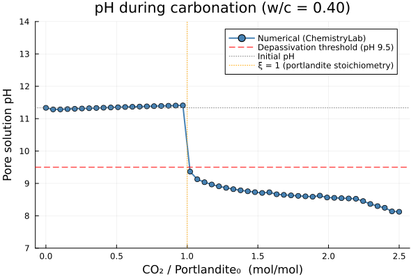

Phase evolution

julia

p2 = plot(
    collect(ξ_range), n_Port_vals ./ n_port0;
    xlabel     = "CO₂ / Portlandite₀  (mol/mol)",
    ylabel     = "Relative amount  (–)",
    label      = "Portlandite  Ca(OH)₂",
    linewidth  = 2,
    marker     = :circle,
    markersize = 4,
    color      = :steelblue,
    title      = "Phase assemblage during carbonation",
    ylims      = (0, 1.05),
    legend     = :topright,
)
plot!(p2, collect(ξ_range), n_Cal_vals   ./ n_port0;
    label     = "Calcite  CaCO₃",
    linewidth = 2, marker = :square, markersize = 4, color = :firebrick,
)
plot!(p2, collect(ξ_range), n_Monoc_vals ./ n_port0;
    label     = "Monocarbonate",
    linewidth = 2, marker = :diamond, markersize = 4, color = :orange,
)
plot!(p2, collect(ξ_range), n_Jen_vals   ./ n_jen0;
    label     = "Jennite (CSH)  – rescaled",
    linewidth = 2, marker = :utriangle, markersize = 4, color = :green,
    linestyle = :dash,
)
vline!(p2, [1.0]; linestyle = :dot, color = :grey, label = "ξ = 1")
p2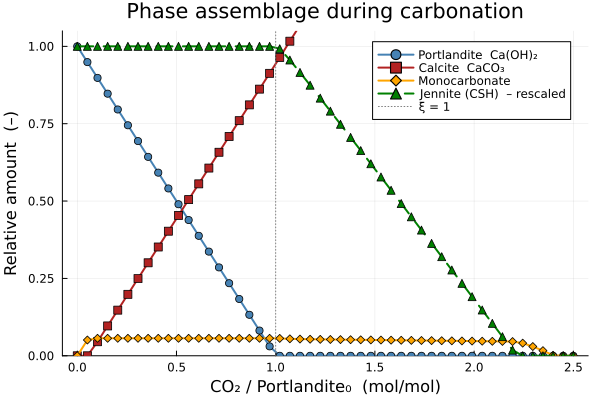

Analysis

The simulation reveals four successive zones as CO₂ uptake increases:

Zone	ξ range	Dominant reaction	pH
I — AFm conversion	0 → ~0.2	monosulphate + CO₂ → monocarbonate + gypsum	≈ 12.5
II — Portlandite buffering	~0.2 → 1	Portlandite + CO₂ → calcite + H₂O	≈ 12.0–12.5
III — Portlandite depletion	ξ ≈ 1	Portlandite exhausted; pH drops sharply	12 → 9.5
IV — CSH decalcification	1 → 2.5	Jennite (CSH) + CO₂ → calcite + amorphous SiO₂·xH₂O	9–10

Key observations:

Zone I: CO₂ first attacks the monosulphate and ettringite, converting them to monocarbonate. pH remains nearly constant because portlandite acts as a reservoir.
Zone II: Once the AFm phases are saturated, portlandite is consumed 1:1 by CO₂ to form calcite. The high solubility of portlandite maintains pH ≈ 12–12.5.
Zone III: The depletion of portlandite at ξ ≈ 1 triggers a sharp pH drop, crossing the steel passivation threshold (9.5). This is the thermodynamic equivalent of the carbonation front passing through the concrete cover.
Zone IV: Above ξ = 1, CSH (Jennite) is decalcified; pH stabilizes around 9–10 before eventually reaching the CO₂/HCO₃⁻ equilibrium (~8.3).

From equilibrium to service life

ChemistryLab provides the thermodynamic driving forces at each CO₂ exposure level. To translate this into a carbonation depth as a function of time, couple the phase diagram above with a diffusion model: the front advances when the local CO₂ concentration exceeds the buffering capacity per unit volume of paste, which is directly read from the ξ-axis at the portlandite depletion point.

Link to the carbonate system

The aqueous speciation within the carbonating pore solution — distribution between CO₂(aq), HCO₃⁻ and CO₃²⁻ — follows the same equilibria described in the CO₂ dissolution example. In the high-pH pore solution (pH > 12), CO₃²⁻ dominates; below pH 8.3, CO₂(aq) takes over.

Carbonation of a Cement Paste ​

System setup ​

Building the equilibrium solver ​

Step 1 — Reference hydrated paste (no CO₂) ​

Step 2 — Progressive CO₂ uptake ​

Results ​

pH of the pore solution ​

Phase evolution ​

Analysis ​

Carbonation of a Cement Paste

System setup

Building the equilibrium solver

Step 1 — Reference hydrated paste (no CO₂)

Step 2 — Progressive CO₂ uptake

Results

pH of the pore solution

Phase evolution

Analysis