
A miscibility gap, and the three answers a formulation can give
The AFm and AFt phases of a Portland cement are binaries — sulfate against hydroxide, sulfate against carbonate — and the Redlich-Kister parameters published for them are strong enough that the mixing energy is concave over an interval. Where an energy is concave the Gibbs minimum is not one composition but two: the phase unmixes, and the equilibrium is a miscibility gap.
This page runs the same cement three ways on the AFm sulfate/hydroxide binary, because the three are genuinely different claims:
ideal mixing — an answer, certified, to a question that was changed;
the published parameters with one composition — the question kept, and the answer is not a minimum. The certificate now says so;
the published parameters with two compositions — the question kept and answered, at the common tangent.
The theory is in the solid-solution chapter; this page is the measurement.
using ChemistryLab
using DynamicQuantities
using OptimaSolver
using OrderedCollections
using Printf
using Plots
default(framestyle = :box, grid = false)

substances = build_species(datapath("cemdata18-thermofun.json"); verbose = false)
byname = Dict(symbol(s) => s for s in substances)
molar_mass(n) = ustrip(us"g/mol", byname[n][:M])
┌───────────────────────────────────────────────────┐
│ Loading database: data/cemdata18-thermofun.json │
└───────────────────────────────────────────────────┘
┌────────────────────┐
│ Building species │
└────────────────────┘
Progress: 82%|███████████████████████████████████████████████████████████████████████████████████████████████████████████████████████████████████▍ | ETA: 0:00:00[K
Progress: 100%|█████████████████████████████████████████████████████████████████████████████████████████████████████████████████████████████████████████████████████████████████| Time: 0:00:00[K1. Where the gap is, before any cement is involved
spinodal_interval scans the second derivative of the molar mixing energy and returns the interval over which it is negative, or nothing when the model is convex. It needs no solve and no system:
RT = 8.31446261815324 * 298.15

models = OrderedDict(
    "ideal" => IdealSolidSolutionModel(),
    "AFm SO4/OH (published)" => RedlichKisterModel(a0 = 0.188RT, a1 = 2.49RT),
    "AFt SO4/CO3 (published)" => RedlichKisterModel(a0 = 1.67RT, a1 = 0.946RT),
    "regular, W = 1.9 RT" => RegularSolutionModel([0.0 1.9RT; 1.9RT 0.0]),
    "regular, W = 2.1 RT" => RegularSolutionModel([0.0 2.1RT; 2.1RT 0.0]),
)

for (label, m) in models
    gap = spinodal_interval(m, 2)
    if gap === nothing
        @printf("  %-26s convex everywhere\n", label)
    else
        @printf("  %-26s concave for x in [%.3f, %.3f]\n", label, gap[1], gap[2])
    end
end
ideal convex everywhere
AFm SO4/OH (published) concave for x in [0.631, 0.914]
AFt SO4/CO3 (published) concave for x in [0.564, 0.830]
regular, W = 1.9 RT convex everywhere
regular, W = 2.1 RT concave for x in [0.391, 0.609]The last two are the classical check: a symmetric regular solution unmixes above W = 2RT exactly, because d²g/dx² at x = ½ is 4 − 2W/RT. The two published cement sets are well past it.
The curve itself makes the shape of the problem visible. A convex energy has one minimum; a concave stretch means the straight line between two compositions lies below the curve, and the system takes the line — which is to say, it takes the two compositions and not any single one between them.
xs = range(0.001, 0.999; length = 400)
g(m, x) = begin
    # molar Gibbs energy of mixing, in units of RT
    ideal = x * log(x) + (1 - x) * log(1 - x)
    excess = if m isa RedlichKisterModel
        x * (1 - x) * (m.a0 + m.a1 * (2x - 1) + m.a2 * (2x - 1)^2) / RT
    else
        0.0
    end
    ideal + excess
end

afm = models["AFm SO4/OH (published)"]
gap = spinodal_interval(afm, 2)

fig = plot(xs, [g(afm, x) for x in xs]; label = "published Redlich-Kister",
           color = :firebrick, linewidth = 2,
           xlabel = "x (sulfate end-member)", ylabel = "g / RT",
           title = "The mixing energy of the AFm sulfate/hydroxide binary",
           size = (760, 420), bottom_margin = 8Plots.mm, left_margin = 8Plots.mm)
plot!(fig, xs, [g(IdealSolidSolutionModel(), x) for x in xs];
      label = "ideal mixing", color = :steelblue, linewidth = 2, linestyle = :dash)
vspan!(fig, [gap[1], gap[2]]; color = :firebrick, alpha = 0.12, label = "spinodal")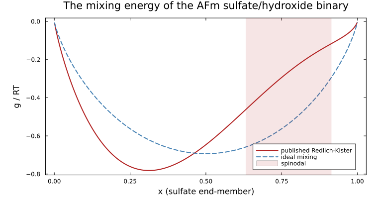
2. The cement, declared three ways
A CEM I paste, with the AFm binary as the only phase whose model changes between the three runs:
CLINKER = OrderedDict("C3S" => 0.65, "C2S" => 0.11, "C3A" => 0.11, "C4AF" => 0.08)
GYPSUM = 0.046
WB = 0.50
BINDER_G = 100.0

pure = split(
    "C3S C2S C3A C4AF Gp Anh Cal Portlandite ettringite monocarbonate " *
    "hemicarbonate C3AH6 C3FH6 straetlingite FeOOHmic AlOHmic Amor-Sl Brc"
)
CSHQ = ["CSHQ-JenD", "CSHQ-JenH", "CSHQ-TobD", "CSHQ-TobH", "KSiOH", "NaSiOH"]
AFM = ["C4AH13", "monosulphate12"]
aqueous = ["SO4-2", "CO2@"]

model = HKFActivityModel(å = 0.0, Ḃ = 0.097637, Kₙ = 0.0)

"""
One system, differing only in how the AFm binary is declared.

`autostart` is a keyword because two of the three cases below are *meant* not to
certify. For those the multi-start cascade -- every backend, then the ideal
pre-solve, then the homotopy continuation -- cannot help: there is no admissible
single-composition minimum for it to find, so it spends minutes arriving at the
answer the first route already gave. The certificate reported is the same one
either way; declining the cascade declines only the search for a better start.
"""
function run_case(afm_phase; autostart = true)
    sp = speciation(substances, vcat(pure, CSHQ, AFM, aqueous);
                    aggregate_state = [AS_AQUEOUS])
    ss = [SolidSolutionPhase("CSHQ", [byname[m] for m in CSHQ]), afm_phase]
    cs = ChemicalSystem(sp, CEMDATA_PRIMARIES; solid_solutions = ss)

    st = ChemicalState(cs)
    for (phase, frac) in CLINKER
        set_quantity!(st, phase,
            BINDER_G * (1 - GYPSUM) * frac / molar_mass(phase) * u"mol")
    end
    set_quantity!(st, "Gp", BINDER_G * GYPSUM / molar_mass("Gp") * u"mol")
    set_quantity!(st, "H2O@", BINDER_G * WB / molar_mass("H2O@") * u"mol")
    b = Float64.(cs.SM.A) * ustrip.(us"mol", st.n)

    eq, cert = equilibrate_certified(st; model = model, b = b, autostart = autostart)
    return cs, eq, cert
end

afm_em = [byname[m] for m in AFM]
published = RedlichKisterModel(a0 = 0.188RT, a1 = 2.49RT)
Case 1 — ideal mixing
cs1, eq1, c1 = run_case(SolidSolutionPhase("AFm_SO4_OH", afm_em))
@printf("optimal=%-5s  worst SI=%+.2e  balance=%.1e  pH=%.4f\n",
        c1.optimal, c1.worst_supersaturation, c1.balance, pH(eq1, model))
┌ Warning: Verbosity toggle: missing_second_order_ad
│ The selected optimization algorithm requires second order derivatives, but `SecondOrder` ADtype was not provided. So a `SecondOrder` with AutoForwardDiff() for both inner and outer will be created, this can be suboptimal and not work in some cases so an explicit `SecondOrder` ADtype is recommended.
└ @ OptimizationBase ~/.julia/packages/OptimizationBase/TvAnm/src/cache.jl:116
optimal=true worst SI=+3.09e-10 balance=2.0e-12 pH=12.5097Case 2 — the published parameters, one composition
SolidSolutionPhase refuses this declaration outright, and names the interval:
err = try
    SolidSolutionPhase("AFm_SO4_OH", afm_em; model = published)
    nothing
catch e
    e
end
println(err.msg)
SolidSolutionPhase "AFm_SO4_OH": the mixing energy of this model is CONCAVE for x in [0.631, 0.914] at T = 298.15 K, so the phase unmixes there: the Gibbs minimum inside that interval is two coexisting compositions, not one, and this formulation has a single amount per species to describe it with. Declare it with `instances = 2` to give it two, which is what a miscibility gap needs; or use ideal mixing, or parameters that keep the energy convex; or pass `check_convexity = false` to proceed with one composition anyway — in which case the optimality certificate no longer proves anything, its sufficiency resting on convexity.Waiving the refusal is what a caller does who believes the answer stays outside the gap. Here it does not, and the certificate is what says so:
cs2, eq2, c2 = run_case(SolidSolutionPhase("AFm_SO4_OH", afm_em;
                                           model = published, check_convexity = false);
                        autostart = false)
@printf("optimal=%-5s  worst SI=%+.2e  balance=%.1e  pH=%.4f\n",
        c2.optimal, c2.worst_supersaturation, c2.balance, pH(eq2, model))
if hasproperty(c2, :worst_violation_split)
    @printf("phases reported as wanting to split: %d   worst split measure %+.2e\n",
            length(c2.split_phases), c2.worst_violation_split)
end
┌ Warning: Verbosity toggle: missing_second_order_ad
│ The selected optimization algorithm requires second order derivatives, but `SecondOrder` ADtype was not provided. So a `SecondOrder` with AutoForwardDiff() for both inner and outer will be created, this can be suboptimal and not work in some cases so an explicit `SecondOrder` ADtype is recommended.
└ @ OptimizationBase ~/.julia/packages/OptimizationBase/TvAnm/src/cache.jl:116
┌ Warning: no route produced a certifiable equilibrium: stationarity 0.00017574700713826215, element balance 1.1679546219056647e-13, worst supersaturation 0.12244470142546326. Automatic initial approximation: declined (autostart = false); returning the answer with the smallest KKT error — audit it with `optimality_certificate`
└ @ ChemistryLab ~/work/ChemistryLab.jl/ChemistryLab.jl/src/equilibrium/certified.jl:845
optimal=false worst SI=+1.22e-01 balance=1.2e-13 pH=12.5097
phases reported as wanting to split: 2 worst split measure +1.22e-01Before the tangent-plane test was applied to phases that are present, this case certified: every member was stationary, nothing absent was supersaturated, and the element balance closed. Stationarity is blind to the one failure that matters for a non-ideal phase — that the minimum is two compositions rather than the one reported — so the answer was a KKT point and not a minimum, and nothing in the output said which.
Case 3 — the published parameters, two compositions
cs3, eq3, c3 = run_case(SolidSolutionPhase("AFm_SO4_OH", afm_em;
                                           model = published, instances = 2);
                        autostart = false)
@printf("optimal=%-5s  worst SI=%+.2e  balance=%.1e  pH=%.4f\n",
        c3.optimal, c3.worst_supersaturation, c3.balance, pH(eq3, model))

n3 = ustrip.(us"mol", eq3.n)
for (grp, ph) in zip(cs3.ss_groups, cs3.solid_solutions)
    startswith(name(ph), "AFm") || continue
    tot = sum(n3[i] for i in grp)
    x = tot > 1.0e-12 ? n3[grp[2]] / tot : NaN
    @printf("  %-14s total %8.5f mol   x(sulfate) = %s\n",
            name(ph), tot, isnan(x) ? "—" : @sprintf("%.4f", x))
end
┌ Warning: Verbosity toggle: missing_second_order_ad
│ The selected optimization algorithm requires second order derivatives, but `SecondOrder` ADtype was not provided. So a `SecondOrder` with AutoForwardDiff() for both inner and outer will be created, this can be suboptimal and not work in some cases so an explicit `SecondOrder` ADtype is recommended.
└ @ OptimizationBase ~/.julia/packages/OptimizationBase/TvAnm/src/cache.jl:116
┌ Warning: no route produced a certifiable equilibrium: stationarity 0.00022872713149862123, element balance 1.837185793170798e-5, worst supersaturation 0.2109373194382007. Automatic initial approximation: declined (autostart = false); returning the answer with the smallest KKT error — audit it with `optimality_certificate`
└ @ ChemistryLab ~/work/ChemistryLab.jl/ChemistryLab.jl/src/equilibrium/certified.jl:845
optimal=false worst SI=+2.11e-01 balance=1.8e-05 pH=12.5161
AFm_SO4_OH total 0.00131 mol x(sulfate) = 0.4902
AFm_SO4_OH#2 total 0.05323 mol x(sulfate) = 0.4902Read that output carefully, because it does not show a common-tangent pair. The two instances come out at the same composition, with the amount split lopsidedly between them, and the certificate still refuses.
That is an honest result, and the page states it rather than dressing it up.
3. The pair itself is computable — the minimization is what does not find it
The two compositions are not unknown. They follow from the mixing model alone, by the construction Glynn and Reardon set out (Glynn and Reardon, 1990) and that PHREEQC uses for a binary solid solution: the pair at which a single straight line is tangent to
ct = common_tangent(published, 2)
sp = spinodal_interval(published, 2)
@printf("common tangent : x = %.4f and %.4f\n", ct[1], ct[2])
@printf("spinodal       : x = %.4f to %.4f  (contained in it, as it must be)\n",
        sp[1], sp[2])
common tangent : x = 0.4999 and 0.9700
spinodal : x = 0.6312 to 0.9142 (contained in it, as it must be)common_tangent solves two equations in two unknowns by Newton and costs microseconds — it involves no chemical system at all. Its answer is checkable without trusting the code: for a symmetric model
A = 3.0                                  # W/RT, well past the threshold of 2
sym = RegularSolutionModel([0.0 A*RT; A*RT 0.0])
a, b = common_tangent(sym, 2)
@printf("symmetric model: x = %.6f and %.6f, and b = 1 - a to %.1e\n",
        a, b, abs(b - (1 - a)))
@printf("residual of  ln(x/(1-x)) + A(1-2x) = 0  :  %+.2e and %+.2e\n",
        log(a / (1 - a)) + A * (1 - 2a), log(b / (1 - b)) + A * (1 - 2b))
symmetric model: x = 0.070720 and 0.929280, and b = 1 - a to 0.0e+00
residual of ln(x/(1-x)) + A(1-2x) = 0 : -2.26e-13 and +2.27e-13So the endpoints of the gap are available to a user who needs them. What does not work is handing them to the minimization as a starting point and expecting it to keep the two lobes apart:
And the split follows, by mass balance
Inside a gap only the proportions move: the two compositions are the same whatever the overall composition is. So once the pair is known, how a given overall composition miscibility_split returns, together with the Gibbs energy the separation releases:
for x̄ in (0.20, 0.40, 0.5268, 0.80, 0.96)
    r = miscibility_split(published, x̄, 2)
    if r.f_beta == 0
        @printf("x̄ = %.4f : homogeneous (outside the pair)\n", x̄)
    else
        # Two calls rather than one: `@printf` takes a LITERAL format string,
        # and `"a" * "b"` is an expression -- `ArgumentError: First argument to
        # @printf after io must be a format string`, raised while the block is
        # lowered, so it kills the build rather than the line.
        @printf("x̄ = %.4f : %.1f %% at x=%.4f and %.1f %% at x=%.4f",
                x̄, 100r.f_alpha, r.x_alpha, 100r.f_beta, r.x_beta)
        @printf("   —  releases %6.1f J/mol   (mass balance %+.0e)\n",
                r.Δg, r.f_alpha * r.x_alpha + r.f_beta * r.x_beta - x̄)
    end
end
x̄ = 0.2000 : homogeneous (outside the pair)
x̄ = 0.4000 : homogeneous (outside the pair)
x̄ = 0.5268 : 94.3 % at x=0.4999 and 5.7 % at x=0.9700 — releases 3.0 J/mol (mass balance +0e+00)
x̄ = 0.8000 : 36.2 % at x=0.4999 and 63.8 % at x=0.9700 — releases 102.8 J/mol (mass balance +0e+00)
x̄ = 0.9600 : 2.1 % at x=0.4999 and 97.9 % at x=0.9700 — releases 2.1 J/mol (mass balance +0e+00)Δg is the distance from the curve down to the common tangent: it says, in joules per mole of binary, how much a single-composition answer overstates the Gibbs energy. The AFm of this paste sits at x̄ = 0.5268, inside the pair, so the figure is not academic.
The one thing the minimization does not deliver
Everything above costs microseconds and needs no solver. What a minimization over two declared instances does not deliver is autostart = false so the seed survives: the second instance empties and the solve stalls at a stationarity of 1.8e-04 where the ideal case reaches 1.1e-15. It is not the starting point — three were tried, including the exact pair — and it is not the iteration budget: between 200 and 5000 iterations the element balance degrades from 1.5e-01 to 4.5e+00. Two instances of one substance put a nearly null direction into the problem, and more iterations walk further along it.
That is also where PHREEQC draws the line: its binary solid-solution calculation is a dedicated construction, not a job handed to the global minimization.
Where this leaves the three questions
| detect a gap | yes — the certificate refuses a single composition inside one, and names the phase |
| locate it | yes — spinodal_interval and common_tangent, from the model alone |
| represent it | yes — instances = 2; the species exist, the groups stay disjoint, conservation is untouched |
| split a given overall composition | yes — miscibility_split, exact, with the energy it releases |
| iterate that back through the aqueous equilibrium | not by minimization over two instances |
The first four are what a user needs to answer "is this phase homogeneous, and if not, into what?". The last is the coupling, and it is the one place this package stops — for a reason that is measured rather than asserted.
Neither GEM-Selektor nor Reaktoro splits a phase by itself either, and PHREEQC draws the same line: it treats a binary solid solution with a dedicated construction rather than handing it to the global minimization.
Stated plainly because a reader deciding whether to trust a number here deserves to know which of these five they are relying on.
Why the second instance is refused for a convex model
Two instances of a convex phase are degenerate: every way of splitting the amount between them has the same energy, so the minimum is a flat manifold and the optimizer is asked to choose a point on it for no reason. Inside a spinodal the common-tangent pair is unique, and the degeneracy does not arise. SolidSolutionPhase therefore admits instances > 1 exactly where spinodal_interval reports a gap.
4. The three answers side by side
labels = ["ideal\nmixing", "published,\none composition", "published,\ntwo compositions"]
certs = [c1, c2, c3]
eqs = [eq1, eq2, eq3]
vols = [ustrip(uconvert(us"cm^3", volume(e).total)) for e in eqs]
phs = [pH(e, model) for e in eqs]
ok = [c.optimal for c in certs]

p1 = bar(labels, vols; legend = false, ylabel = "total volume (cm³)",
         color = [o ? :seagreen : :firebrick for o in ok], title = "Volume")
p2 = bar(labels, phs; legend = false, ylabel = "pH", title = "Pore solution pH",
         color = [o ? :seagreen : :firebrick for o in ok],
         ylims = (12.5, 13.5))
fig3 = plot(p1, p2; layout = (1, 2), size = (900, 420),
            bottom_margin = 16Plots.mm, left_margin = 8Plots.mm)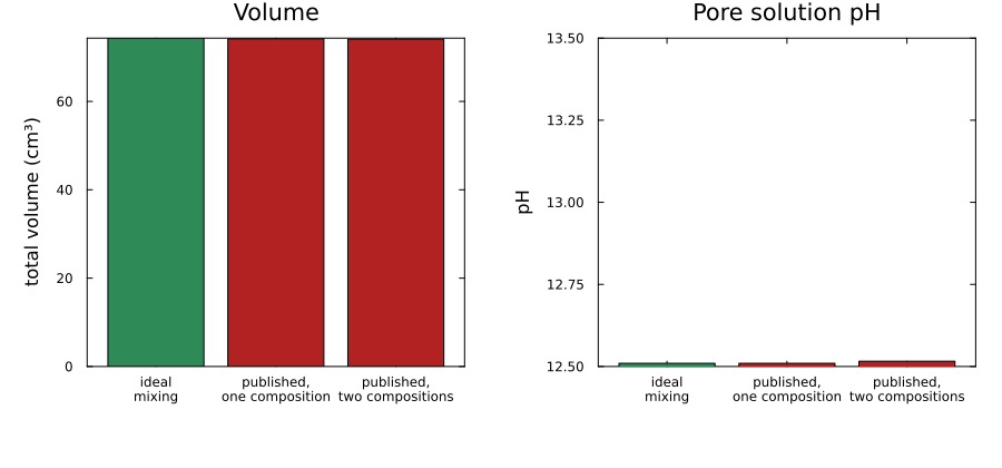
Green is a proof and red is its absence — not a claim that a red bar is far from the truth, which nothing here establishes. The point of the middle case is precisely that it looks like the others: same pH to four figures, element balance at 2e-14, a perfectly ordinary-looking assemblage. Only the certificate tells it apart, and only since it learned to test a phase that is present.
What this does and does not settle
optimal = true in case 3 is a proof of a KKT point at which no present phase wants to split and no absent phase is supersaturated. For a convex problem those conditions are sufficient for a global minimum, and that is why the certificate means what it means on every other page. With a concave mixing model the problem is no longer convex, so global optimality is not implied by stationarity alone — what the certificate adds here is the tangent-plane test, which is exactly the condition that separates a common-tangent pair from a spurious stationary point.
Case 3 does not reach that state here, so nothing in this page is offered as a certified non-convex answer. What the page establishes is narrower and solid: the criterion detects the gap, the refusal names it, and the representation exists for a solver that can use it.
5. How other codes represent the same thing
GEM-Selektor computes the same criterion — its phase stability index Ω and phase_split_measure compute, derived independently from the same KKT conditions (Kulik et al., 2013). Where the two differ is not detection but declaration: CEMDATA18 ships the AFm and AFt binaries under two names each, so a GEMS user represents a gap by declaring the binary twice, in the database. instances = 2 is the same representation asked for by a keyword instead.
Neither code splits a phase by itself. A GEMS user gets the right answer because the database ships the binary twice and the solver is handed two declarations to populate; here the declarations exist and the solver still has to be told to look in the other lobe. That is the honest statement of where things stand, and the remaining gap is the same one in both: nothing decides, on its own, that a phase should be split in two.