CO₂ Dissolution and the Carbonate System

The carbonate system — CO₂(aq) / HCO₃⁻ / CO₃²⁻ — is one of the most important chemical equilibria in natural water chemistry, geochemistry, and environmental science. It controls the pH of rainwater, rivers, oceans, and aquifers, and governs the dissolution and precipitation of carbonate minerals such as calcite and dolomite.

This example shows how to:

Load species from a thermodynamic database and build a ChemicalSystem.
Extract dissociation constants (pKₐ₁, pKₐ₂) directly from standard Gibbs energies.
Simulate CO₂ dissolution in pure water over several orders of magnitude.
Construct the analytical speciation diagram (fraction of each carbonate species vs pH).

System setup

All species are loaded from the SLOP98 inorganic database. The system contains only H, O, C and charge-bearing species; no other elements are needed.

Symbol	Species	Phase
`H2O@`	H₂O — water	aqueous solvent
`H+`	H⁺ — proton	aqueous solute
`OH-`	OH⁻ — hydroxide	aqueous solute
`CO2@`	CO₂(aq) — dissolved CO₂	aqueous solute
`HCO3-`	HCO₃⁻ — bicarbonate	aqueous solute
`CO3-2`	CO₃²⁻ — carbonate	aqueous solute

The three primary species H2O@, H+, CO3-2 form a basis for the whole system: every other aqueous species is a linear combination of these three.

julia

using Optimization, OptimizationIpopt
using ChemistryLab
using DynamicQuantities

substances = build_species(datapath("slop98-inorganic-thermofun.json"))

# Select only the six carbonate-system species
dict = Dict(symbol(s) => s for s in substances)
species = [dict[sym] for sym in split("H2O@ H+ OH- CO2@ HCO3- CO3-2")]

cs = ChemicalSystem(species, ["H2O@", "H+", "CO3-2"])

┌──────────────────────────────────────────────────────────┐
│  Loading database: data/slop98-inorganic-thermofun.json  │
└──────────────────────────────────────────────────────────┘
┌────────────────────┐
│  Building species  │
└────────────────────┘

Progress:  23%|█████████████████████████████████████▉                                                                                                                           |  ETA: 0:00:00[K
Progress:  47%|████████████████████████████████████████████████████████████████████████████▏                                                                                    |  ETA: 0:00:00[K
Progress:  71%|██████████████████████████████████████████████████████████████████████████████████████████████████████████████████▍                                              |  ETA: 0:00:00[K
Progress:  94%|███████████████████████████████████████████████████████████████████████████████████████████████████████████████████████████████████████████████████████▉         |  ETA: 0:00:00[K
Progress: 100%|█████████████████████████████████████████████████████████████████████████████████████████████████████████████████████████████████████████████████████████████████| Time: 0:00:00[K

The chemical system in full

julia

cs

6-element ChemicalSystem{Species{Int64}, AbstractReaction, StoichMatrix{Int64, Symbol, Vector{Symbol}, Matrix{Int64}, Species{Int64}}, StoichMatrix{Int64, Species{Int64}, Vector{Species{Int64}}, Matrix{Int64}, Species{Int64}}, Nothing}:
 H2O@ {Water HGK} [H2O@ ◆ H₂O@]
 H+ {H+} [H+ ◆ H⁺]
 OH- {OH- hydroXyl ion} [OH- ◆ OH⁻]
 CO2@ {CO2,aq (+ H2O = H2CO3,aq )} [CO2@ ◆ CO₂@]
 HCO3- {HCO3- bicarbonate ion} [HCO3- ◆ HCO₃⁻]
 CO3-2 {CO3-2 carbonate ion} [CO3-2 ◆ CO₃²⁻]

Larger carbonate systems

If calcium is relevant (e.g. hard water, calcite dissolution), add Ca+2 and its complexes to the species list and extend the primaries to ["H2O@", "H+", "CO3-2", "Ca+2"]. The SLOP98 inorganic database also contains Ca(HCO3)+ and Ca(CO3)@.

Dissociation constants from thermodynamic data

The two acid–base equilibria of the carbonate system are:

Both constants are computed from standard Gibbs energies of formation at 25 °C, exactly as in the acetic acid titration example:

julia

R  = ustrip(Constants.R)
T  = 298.15   # K
RT = R * T

sp = Dict(symbol(s) => s for s in cs.species)

# pKa1 : CO₂(aq) + H2O ⇌  HCO₃⁻ + H⁺
Ka1  = exp(-(sp["HCO3-"].ΔₐG⁰(T = T) + sp["H+"].ΔₐG⁰(T = T) - sp["H2O@"].ΔₐG⁰(T = T) - sp["CO2@"].ΔₐG⁰(T = T)) / RT)
pKa1 = -log10(Ka1)

# pKa2 : HCO₃⁻ ⇌ H⁺ + CO₃²⁻
Ka2  = exp(-(sp["CO3-2"].ΔₐG⁰(T = T) + sp["H+"].ΔₐG⁰(T = T) - sp["HCO3-"].ΔₐG⁰(T = T)) / RT)
pKa2 = -log10(Ka2)

# pKw : H₂O ⇌ H⁺ + OH⁻
Kw   = exp(-(sp["H+"].ΔₐG⁰(T = T) + sp["OH-"].ΔₐG⁰(T = T) - sp["H2O@"].ΔₐG⁰(T = T)) / RT)
pKw  = -log10(Kw)

println("pKa1 (CO₂(aq) / HCO₃⁻) = ", round(pKa1, digits = 2), "   (lit. 6.35)")
println("pKa2 (HCO₃⁻  / CO₃²⁻)  = ", round(pKa2, digits = 2), "   (lit. 10.33)")
println("pKw  (H₂O    / H⁺+OH⁻) = ", round(pKw,  digits = 2), "   (lit. 14.00)")

pKa1 (CO₂(aq) / HCO₃⁻) = 6.34   (lit. 6.35)
pKa2 (HCO₃⁻  / CO₃²⁻)  = 10.33   (lit. 10.33)
pKw  (H₂O    / H⁺+OH⁻) = 14.0   (lit. 14.00)

Building the equilibrium solver

A single EquilibriumSolver is compiled once and reused for every point of the scan:

julia

using Optimization, OptimizationIpopt

solver = EquilibriumSolver(
    cs,
    DiluteSolutionModel(),
    IpoptOptimizer(
        acceptable_tol        = 1e-10,
        dual_inf_tol          = 1e-10,
        acceptable_iter       = 1000,
        constr_viol_tol       = 1e-10,
        warm_start_init_point = "no",
    );
    variable_space = Val(:linear),
    abstol  = 1e-8,
    reltol  = 1e-8,
)

EquilibriumSolver{ChemistryLab.var"#μ#build_potentials##0"{ChemistryLab.var"#lna#activity_model##2"{Nothing, Bool, Bool, Vector{Vector{Int64}}, Float64, Vector{Int64}, Vector{Int64}, Int64, Bool}}, IpoptOptimizer, Val{:linear}, DiluteSolutionModel}(ChemistryLab.var"#μ#build_potentials##0"{ChemistryLab.var"#lna#activity_model##2"{Nothing, Bool, Bool, Vector{Vector{Int64}}, Float64, Vector{Int64}, Vector{Int64}, Int64, Bool}}(ChemistryLab.var"#lna#activity_model##2"{Nothing, Bool, Bool, Vector{Vector{Int64}}, Float64, Vector{Int64}, Vector{Int64}, Int64, Bool}(nothing, false, false, Vector{Int64}[], 4.016550535127659, Int64[], [2, 3, 4, 5, 6], 1, true)), IpoptOptimizer(1.0e-10, 1000, 1.0e-10, 1.0e-10, 0.0001, "no", "no", "mumps", "none", "", "", "yes", "gradient-based", 100.0, "no", "no", "monotone", "quality-function", 0.1, "obj-constr-filter", "no", "exact", 6, "bfgs", "no", "filter", "no", Dict{String, Any}()), Val{:linear}(), Base.Pairs(:abstol => 1.0e-8, :reltol => 1.0e-8), DiluteSolutionModel())

CO₂ dissolution scan

The experiment: 1 kg of pure water receives an increasing amount of dissolved CO₂ (CO₂(aq)), from trace atmospheric levels (~10⁻⁵ mol) up to a highly carbonated solution (~0.1 mol). Three representative concentrations illustrate the pH trend:

julia

s = ChemicalState(cs)
for (n_CO2, label) in [
    (1e-5, "atmospheric, ~400 ppm"),
    (1e-3, "lightly carbonated"),
    (1e-1, "strongly carbonated"),
]
    set_quantity!(s, "H2O@", 1.0u"kg")
    set_quantity!(s, "CO2@", n_CO2 * u"mol")
    V_liq = volume(s).liquid
    set_quantity!(s, "H+",  1e-7u"mol/L" * V_liq)
    set_quantity!(s, "OH-", 1e-7u"mol/L" * V_liq)
    s_eq = solve(solver, s)
    println("pH at [CO₂]₀ = ", n_CO2, " mol (", label, ") : ",
            round(pH(s_eq), digits = 2))
end

┌ Warning: Verbosity toggle: missing_second_order_ad
│  The selected optimization algorithm requires second order derivatives, but `SecondOrder` ADtype was not provided. So a `SecondOrder` with AutoForwardDiff() for both inner and outer will be created, this can be suboptimal and not work in some cases so an explicit `SecondOrder` ADtype is recommended.
└ @ OptimizationBase ~/.julia/packages/OptimizationBase/TvAnm/src/cache.jl:116
┌ Info: Verbosity toggle: unsupported_kwargs
└  common abstol is currently not used by IpoptOptimizer(1.0e-10, 1000, 1.0e-10, 1.0e-10, 0.0001, "no", "no", "mumps", "none", "", "", "yes", "gradient-based", 100.0, "no", "no", "monotone", "quality-function", 0.1, "obj-constr-filter", "no", "exact", 6, "bfgs", "no", "filter", "no", Dict{String, Any}())
This is Ipopt version 3.14.19, running with linear solver MUMPS 5.9.0.

Number of nonzeros in equality constraint Jacobian...:       18
Number of nonzeros in inequality constraint Jacobian.:        0
Number of nonzeros in Lagrangian Hessian.............:       21

Total number of variables............................:        6
                     variables with only lower bounds:        0
                variables with lower and upper bounds:        6
                     variables with only upper bounds:        0
Total number of equality constraints.................:        3
Total number of inequality constraints...............:        0
        inequality constraints with only lower bounds:        0
   inequality constraints with lower and upper bounds:        0
        inequality constraints with only upper bounds:        0

iter    objective    inf_pr   inf_du lg(mu)  ||d||  lg(rg) alpha_du alpha_pr  ls
   0 -5.3180181e+03 3.00e-02 3.68e+00  -1.0 0.00e+00    -  0.00e+00 0.00e+00   0
   1 -5.3135923e+03 1.37e-02 5.93e+00  -1.0 5.65e-02    -  9.91e-01 5.44e-01h  1
   2 -5.3120214e+03 6.82e-03 4.17e+01  -1.0 1.78e-02    -  1.00e+00 5.02e-01h  1
   3 -5.3112398e+03 3.17e-03 4.71e+01  -1.0 6.06e-03    -  1.00e+00 5.35e-01h  1
   4 -5.3107385e+03 8.52e-04 4.98e+01  -1.0 4.46e-03    -  1.00e+00 7.31e-01h  1
   5 -5.3106460e+03 4.40e-04 2.20e+02  -1.0 1.72e-03    -  1.00e+00 4.83e-01h  1
   6 -5.3105768e+03 1.27e-04 2.59e+02  -1.0 5.92e-04    -  1.00e+00 7.11e-01h  1
   7 -5.3105626e+03 6.53e-05 1.22e+03  -1.0 2.56e-04    -  1.00e+00 4.87e-01h  1
   8 -5.3105513e+03 1.50e-05 1.10e+03  -1.0 8.64e-05    -  1.00e+00 7.70e-01h  1
   9 -5.3105503e+03 1.06e-05 7.32e+03  -1.0 3.78e-05    -  1.00e+00 2.93e-01f  2
iter    objective    inf_pr   inf_du lg(mu)  ||d||  lg(rg) alpha_du alpha_pr  ls
  10 -5.3105479e+03 6.64e-19 4.22e-01  -1.0 1.25e-05    -  1.00e+00 1.00e+00h  1
  11 -5.3110206e+03 2.20e-18 6.02e-01  -3.8 2.05e-02    -  1.00e+00 1.00e+00f  1
  12 -5.3110447e+03 1.36e-19 2.55e-01  -3.8 1.31e-03    -  1.00e+00 1.00e+00f  1
  13 -5.3110492e+03 2.71e-20 2.17e-01  -3.8 2.89e-04    -  1.00e+00 1.00e+00f  1
  14 -5.3110497e+03 3.39e-21 3.80e-02  -3.8 4.05e-05    -  1.00e+00 1.00e+00f  1
  15 -5.3110498e+03 7.11e-15 7.89e-04  -3.8 4.08e-06    -  1.00e+00 1.00e+00f  1
  16 -5.3110504e+03 7.11e-15 5.66e-01  -5.7 5.44e-05    -  9.90e-01 1.00e+00f  1
  17 -5.3110505e+03 0.00e+00 5.55e-01  -5.7 7.40e-06    -  1.00e+00 1.00e+00f  1
  18 -5.3110505e+03 0.00e+00 9.85e-02  -5.7 2.01e-06    -  1.00e+00 1.00e+00f  1
  19 -5.3110505e+03 0.00e+00 1.57e-03  -5.7 3.65e-07    -  1.00e+00 1.00e+00f  1
iter    objective    inf_pr   inf_du lg(mu)  ||d||  lg(rg) alpha_du alpha_pr  ls
  20 -5.3110505e+03 0.00e+00 1.99e-06  -5.7 7.49e-09    -  1.00e+00 1.00e+00f  1
  21 -5.3110505e+03 7.11e-15 4.35e-01  -8.6 2.32e-06    -  8.54e-01 1.00e+00f  1
  22 -5.3110505e+03 1.42e-14 2.43e-01  -8.6 7.06e-07    -  1.00e+00 1.00e+00f  1
  23 -5.3110505e+03 7.11e-15 2.25e-01  -8.6 1.80e-07    -  1.00e+00 1.00e+00h  1
  24 -5.3110505e+03 7.11e-15 9.06e-02  -8.6 1.76e-08    -  1.00e+00 1.00e+00h  1
  25 -5.3110505e+03 0.00e+00 1.08e-02  -8.6 2.65e-09    -  1.00e+00 1.00e+00h  1
  26 -5.3110505e+03 0.00e+00 1.99e-04  -8.6 3.46e-10    -  1.00e+00 1.00e+00f  1
  27 -5.3110505e+03 0.00e+00 1.17e-07  -8.6 8.18e-12    -  1.00e+00 1.00e+00f  1
  28 -5.3110505e+03 1.69e-21 3.61e-14  -8.6 4.60e-15    -  1.00e+00 1.00e+00f  1

Number of Iterations....: 28

                                   (scaled)                 (unscaled)
Objective...............:  -1.9411001047780564e+03   -5.3110505074890680e+03
Dual infeasibility......:   3.6132157351628074e-14    9.8861316923673420e-14
Constraint violation....:   1.6940658945086007e-21    1.6940658945086007e-21
Variable bound violation:   0.0000000000000000e+00    0.0000000000000000e+00
Complementarity.........:   2.5059035596813542e-09    6.8564111349043764e-09
Overall NLP error.......:   2.5059035596813542e-09    6.8564111349043764e-09


Number of objective function evaluations             = 30
Number of objective gradient evaluations             = 29
Number of equality constraint evaluations            = 30
Number of inequality constraint evaluations          = 0
Number of equality constraint Jacobian evaluations   = 29
Number of inequality constraint Jacobian evaluations = 0
Number of Lagrangian Hessian evaluations             = 28
Total seconds in IPOPT                               = 5.080

EXIT: Optimal Solution Found.
pH at [CO₂]₀ = 1.0e-5 mol (atmospheric, ~400 ppm) : 5.72
┌ Warning: Verbosity toggle: missing_second_order_ad
│  The selected optimization algorithm requires second order derivatives, but `SecondOrder` ADtype was not provided. So a `SecondOrder` with AutoForwardDiff() for both inner and outer will be created, this can be suboptimal and not work in some cases so an explicit `SecondOrder` ADtype is recommended.
└ @ OptimizationBase ~/.julia/packages/OptimizationBase/TvAnm/src/cache.jl:116
┌ Info: Verbosity toggle: unsupported_kwargs
└  common abstol is currently not used by IpoptOptimizer(1.0e-10, 1000, 1.0e-10, 1.0e-10, 0.0001, "no", "no", "mumps", "none", "", "", "yes", "gradient-based", 100.0, "no", "no", "monotone", "quality-function", 0.1, "obj-constr-filter", "no", "exact", 6, "bfgs", "no", "filter", "no", Dict{String, Any}())
This is Ipopt version 3.14.19, running with linear solver MUMPS 5.9.0.

Number of nonzeros in equality constraint Jacobian...:       18
Number of nonzeros in inequality constraint Jacobian.:        0
Number of nonzeros in Lagrangian Hessian.............:       21

Total number of variables............................:        6
                     variables with only lower bounds:        0
                variables with lower and upper bounds:        6
                     variables with only upper bounds:        0
Total number of equality constraints.................:        3
Total number of inequality constraints...............:        0
        inequality constraints with only lower bounds:        0
   inequality constraints with lower and upper bounds:        0
        inequality constraints with only upper bounds:        0

iter    objective    inf_pr   inf_du lg(mu)  ||d||  lg(rg) alpha_du alpha_pr  ls
   0 -5.3180181e+03 2.90e-02 3.68e+00  -1.0 0.00e+00    -  0.00e+00 0.00e+00   0
   1 -5.3136590e+03 1.32e-02 5.90e+00  -1.0 5.67e-02    -  9.91e-01 5.46e-01h  1
   2 -5.3120434e+03 6.16e-03 4.02e+01  -1.0 1.71e-02    -  1.00e+00 5.32e-01h  1
   3 -5.3112552e+03 2.50e-03 3.90e+01  -1.0 5.78e-03    -  1.00e+00 5.95e-01h  1
   4 -5.3107412e+03 1.32e-04 1.87e+01  -1.0 3.82e-03    -  1.00e+00 9.47e-01h  1
   5 -5.3107140e+03 2.45e-05 3.80e+01  -1.0 1.31e-03    -  1.00e+00 8.14e-01f  1
   6 -5.3107092e+03 1.73e-18 9.77e+00  -1.0 3.25e-04    -  1.00e+00 1.00e+00f  1
   7 -5.3107091e+03 7.11e-15 8.99e-06  -1.0 6.25e-06    -  1.00e+00 1.00e+00f  1
   8 -5.3111708e+03 7.11e-15 5.79e-01  -2.5 2.00e-02    -  1.00e+00 1.00e+00f  1
   9 -5.3111933e+03 0.00e+00 1.15e-01  -2.5 1.20e-03    -  1.00e+00 1.00e+00f  1
iter    objective    inf_pr   inf_du lg(mu)  ||d||  lg(rg) alpha_du alpha_pr  ls
  10 -5.3111957e+03 4.34e-19 5.16e-03  -2.5 1.47e-04    -  1.00e+00 1.00e+00f  1
  11 -5.3112079e+03 4.34e-19 2.82e+00  -3.8 7.71e-04    -  8.68e-01 9.96e-01f  1
  12 -5.3112111e+03 4.34e-19 1.14e+02  -3.8 4.06e-04    -  1.00e+00 1.00e+00f  1
  13 -5.3112113e+03 7.11e-15 7.95e-03  -3.8 3.37e-05    -  1.00e+00 1.00e+00f  1
  14 -5.3112113e+03 0.00e+00 7.11e-03  -3.8 6.11e-06    -  1.00e+00 1.00e+00f  1
  15 -5.3112113e+03 0.00e+00 1.62e-06  -3.8 1.12e-07    -  1.00e+00 1.00e+00f  1
  16 -5.3112123e+03 7.11e-15 5.50e-01  -5.7 1.54e-04    -  9.05e-01 1.00e+00f  1
  17 -5.3112124e+03 0.00e+00 1.86e-01  -5.7 3.14e-05    -  1.00e+00 1.00e+00f  1
  18 -5.3112125e+03 7.11e-15 5.65e-02  -5.7 1.12e-05    -  1.00e+00 1.00e+00f  1
  19 -5.3112125e+03 7.11e-15 1.17e-03  -5.7 2.22e-06    -  1.00e+00 1.00e+00f  1
iter    objective    inf_pr   inf_du lg(mu)  ||d||  lg(rg) alpha_du alpha_pr  ls
  20 -5.3112125e+03 7.11e-15 6.91e-06  -5.7 1.55e-07    -  1.00e+00 1.00e+00h  1
  21 -5.3112125e+03 0.00e+00 5.01e-01  -8.6 4.92e-06    -  9.97e-01 1.00e+00f  1
  22 -5.3112125e+03 2.17e-19 2.18e-01  -8.6 4.13e-07    -  1.00e+00 1.00e+00f  1
  23 -5.3112125e+03 2.17e-19 2.05e-01  -8.6 2.80e-08    -  1.00e+00 1.00e+00f  1
  24 -5.3112125e+03 7.11e-15 6.29e-02  -8.6 4.01e-09    -  1.00e+00 1.00e+00f  1
  25 -5.3112125e+03 7.11e-15 8.81e-03  -8.6 8.92e-10    -  1.00e+00 1.00e+00h  1
  26 -5.3112125e+03 0.00e+00 1.03e-04  -8.6 8.20e-11    -  1.00e+00 1.00e+00h  1
  27 -5.3112125e+03 7.11e-15 1.51e-08  -8.6 9.78e-13    -  1.00e+00 1.00e+00f  1
  28 -5.3112125e+03 7.11e-15 7.88e-02  -9.0 5.94e-09    -  1.00e+00 1.00e+00h  1
  29 -5.3112125e+03 4.34e-19 1.15e-03  -9.0 1.39e-10    -  1.00e+00 1.00e+00h  1
iter    objective    inf_pr   inf_du lg(mu)  ||d||  lg(rg) alpha_du alpha_pr  ls
  30 -5.3112125e+03 7.11e-15 5.41e-06  -9.0 9.78e-12    -  1.00e+00 1.00e+00h  1
  31 -5.3112125e+03 7.11e-15 2.70e-11  -9.0 2.18e-14    -  1.00e+00 1.00e+00h  1

Number of Iterations....: 31

                                   (scaled)                 (unscaled)
Objective...............:  -1.9411592999211866e+03   -5.3112124715187374e+03
Dual infeasibility......:   2.7025287523590822e-11    7.3943979841068725e-11
Constraint violation....:   7.1054273576010019e-15    7.1054273576010019e-15
Variable bound violation:   0.0000000000000000e+00    0.0000000000000000e+00
Complementarity.........:   9.0909090930547954e-10    2.4873666862083962e-09
Overall NLP error.......:   9.0909090930547954e-10    2.4873666862083962e-09


Number of objective function evaluations             = 32
Number of objective gradient evaluations             = 32
Number of equality constraint evaluations            = 32
Number of inequality constraint evaluations          = 0
Number of equality constraint Jacobian evaluations   = 32
Number of inequality constraint Jacobian evaluations = 0
Number of Lagrangian Hessian evaluations             = 31
Total seconds in IPOPT                               = 0.003

EXIT: Optimal Solution Found.
pH at [CO₂]₀ = 0.001 mol (lightly carbonated) : 4.68
┌ Warning: Verbosity toggle: missing_second_order_ad
│  The selected optimization algorithm requires second order derivatives, but `SecondOrder` ADtype was not provided. So a `SecondOrder` with AutoForwardDiff() for both inner and outer will be created, this can be suboptimal and not work in some cases so an explicit `SecondOrder` ADtype is recommended.
└ @ OptimizationBase ~/.julia/packages/OptimizationBase/TvAnm/src/cache.jl:116
┌ Info: Verbosity toggle: unsupported_kwargs
└  common abstol is currently not used by IpoptOptimizer(1.0e-10, 1000, 1.0e-10, 1.0e-10, 0.0001, "no", "no", "mumps", "none", "", "", "yes", "gradient-based", 100.0, "no", "no", "monotone", "quality-function", 0.1, "obj-constr-filter", "no", "exact", 6, "bfgs", "no", "filter", "no", Dict{String, Any}())
This is Ipopt version 3.14.19, running with linear solver MUMPS 5.9.0.

Number of nonzeros in equality constraint Jacobian...:       18
Number of nonzeros in inequality constraint Jacobian.:        0
Number of nonzeros in Lagrangian Hessian.............:       21

Total number of variables............................:        6
                     variables with only lower bounds:        0
                variables with lower and upper bounds:        6
                     variables with only upper bounds:        0
Total number of equality constraints.................:        3
Total number of inequality constraints...............:        0
        inequality constraints with only lower bounds:        0
   inequality constraints with lower and upper bounds:        0
        inequality constraints with only upper bounds:        0

iter    objective    inf_pr   inf_du lg(mu)  ||d||  lg(rg) alpha_du alpha_pr  ls
   0 -5.3323052e+03 2.00e-02 3.51e+00  -1.0 0.00e+00    -  0.00e+00 0.00e+00   0
   1 -5.3257981e+03 0.00e+00 1.81e+00  -1.0 7.84e-02    -  9.90e-01 1.00e+00h  1
   2 -5.3260555e+03 7.11e-15 4.58e-01  -1.0 2.22e-02    -  1.00e+00 1.00e+00f  1
   3 -5.3266417e+03 7.11e-15 3.36e-01  -1.7 3.53e-02    -  8.91e-01 1.00e+00f  1
   4 -5.3267666e+03 0.00e+00 7.18e-02  -1.7 1.25e-02    -  1.00e+00 1.00e+00f  1
   5 -5.3269102e+03 7.11e-15 3.06e-01  -2.5 1.21e-02    -  1.00e+00 1.00e+00f  1
   6 -5.3269238e+03 7.11e-15 3.06e-02  -2.5 1.82e-03    -  1.00e+00 1.00e+00f  1
   7 -5.3269252e+03 0.00e+00 1.35e-03  -2.5 2.40e-04    -  1.00e+00 1.00e+00f  1
   8 -5.3269466e+03 0.00e+00 4.51e-01  -3.8 2.68e-03    -  1.00e+00 1.00e+00f  1
   9 -5.3269481e+03 0.00e+00 5.22e-02  -3.8 3.67e-04    -  1.00e+00 1.00e+00f  1
iter    objective    inf_pr   inf_du lg(mu)  ||d||  lg(rg) alpha_du alpha_pr  ls
  10 -5.3269484e+03 7.11e-15 6.47e-03  -3.8 1.07e-04    -  1.00e+00 1.00e+00f  1
  11 -5.3269484e+03 0.00e+00 7.87e-05  -3.8 9.51e-06    -  1.00e+00 1.00e+00f  1
  12 -5.3269494e+03 7.11e-15 5.54e-01  -5.7 2.66e-04    -  1.00e+00 1.00e+00f  1
  13 -5.3269494e+03 2.78e-17 1.71e-01  -5.7 4.48e-05    -  1.00e+00 1.00e+00f  1
  14 -5.3269494e+03 7.11e-15 3.60e-02  -5.7 9.60e-06    -  1.00e+00 1.00e+00f  1
  15 -5.3269494e+03 2.78e-17 3.06e-04  -5.7 3.35e-07    -  1.00e+00 1.00e+00h  1
  16 -5.3269494e+03 7.11e-15 4.26e-08  -5.7 8.22e-10    -  1.00e+00 1.00e+00h  1
  17 -5.3269494e+03 7.11e-15 5.19e-01  -8.6 5.65e-06    -  1.00e+00 1.00e+00f  1
  18 -5.3269494e+03 7.11e-15 2.13e-01  -8.6 1.13e-07    -  1.00e+00 1.00e+00f  1
  19 -5.3269494e+03 0.00e+00 2.04e-01  -8.6 1.54e-08    -  1.00e+00 1.00e+00h  1
iter    objective    inf_pr   inf_du lg(mu)  ||d||  lg(rg) alpha_du alpha_pr  ls
  20 -5.3269494e+03 7.11e-15 5.95e-02  -8.6 2.78e-09    -  1.00e+00 1.00e+00f  1
  21 -5.3269494e+03 1.39e-17 4.30e-03  -8.6 4.61e-10    -  1.00e+00 1.00e+00h  1
  22 -5.3269494e+03 0.00e+00 1.34e-05  -8.6 2.30e-11    -  1.00e+00 1.00e+00h  1
  23 -5.3269494e+03 7.11e-15 1.54e-10  -8.6 7.75e-14    -  1.00e+00 1.00e+00f  1
  24 -5.3269494e+03 7.11e-15 7.88e-02  -9.0 5.76e-09    -  1.00e+00 1.00e+00h  1
  25 -5.3269494e+03 0.00e+00 1.15e-03  -9.0 9.92e-11    -  1.00e+00 1.00e+00h  1
  26 -5.3269494e+03 2.78e-17 5.20e-06  -9.0 6.29e-12    -  1.00e+00 1.00e+00f  1
  27 -5.3269494e+03 7.11e-15 1.02e-11  -9.0 8.77e-15    -  1.00e+00 1.00e+00h  1

Number of Iterations....: 27

                                   (scaled)                 (unscaled)
Objective...............:  -1.9469108948743378e+03   -5.3269494297619594e+03
Dual infeasibility......:   1.0182960547856023e-11    2.7861632510506506e-11
Constraint violation....:   7.1054273576010019e-15    7.1054273576010019e-15
Variable bound violation:   0.0000000000000000e+00    0.0000000000000000e+00
Complementarity.........:   9.0909090913741123e-10    2.4873666857485442e-09
Overall NLP error.......:   9.0909090913741123e-10    2.4873666857485442e-09


Number of objective function evaluations             = 28
Number of objective gradient evaluations             = 28
Number of equality constraint evaluations            = 28
Number of inequality constraint evaluations          = 0
Number of equality constraint Jacobian evaluations   = 28
Number of inequality constraint Jacobian evaluations = 0
Number of Lagrangian Hessian evaluations             = 27
Total seconds in IPOPT                               = 0.003

EXIT: Optimal Solution Found.
pH at [CO₂]₀ = 0.1 mol (strongly carbonated) : 3.68

For the full scan used to generate the plots below, loop over 60 log-spaced points:

julia

sp_idx = Dict(symbol(s) => i for (i, s) in enumerate(cs.species))

n_CO2_range = exp.(range(log(1e-5), log(0.1); length = 60))   # mol, in 1 kg H₂O

pH_vals     = Float64[]
f_CO2_vals  = Float64[]
f_HCO3_vals = Float64[]
f_CO3_vals  = Float64[]

s = ChemicalState(cs)
for n_CO2 in n_CO2_range
    set_quantity!(s, "H2O@",  1.0u"kg")
    set_quantity!(s, "CO2@",  n_CO2 * u"mol")

    V_liq = volume(s).liquid
    set_quantity!(s, "H+",  1e-7u"mol/L" * V_liq)   # pH-neutral seed
    set_quantity!(s, "OH-", 1e-7u"mol/L" * V_liq)

    s_eq = solve(solver, s)
    push!(pH_vals, pH(s_eq))

    n_a = ustrip(s_eq.n[sp_idx["CO2@"]])
    n_b = ustrip(s_eq.n[sp_idx["HCO3-"]])
    n_c = ustrip(s_eq.n[sp_idx["CO3-2"]])
    n_C = n_a + n_b + n_c

    push!(f_CO2_vals,  n_a / n_C)
    push!(f_HCO3_vals, n_b / n_C)
    push!(f_CO3_vals,  n_c / n_C)
end

Result: pH as a function of dissolved CO₂

julia

using Plots

p1 = plot(
    log10.(n_CO2_range), pH_vals;
    xlabel    = "log₁₀([CO₂]₀) (mol/L)",
    ylabel    = "Equilibrium pH",
    label     = "Numerical (ChemistryLab)",
    linewidth = 2,
    marker    = :circle,
    markersize = 3,
    color     = :steelblue,
    title     = "CO₂ dissolution in pure water (25 °C)",
    ylims     = (3, 7),
    legend    = :right,
)
hline!(p1, [pKa1]; linestyle = :dot, color = :orange, label = "pKa1 = $(round(pKa1, digits=2))")
vline!(p1, [log10(1.4e-5)]; linestyle = :dash, color = :grey,
       label = "Atmospheric CO₂ (~400 ppm)")
p1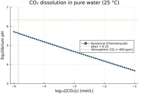

Speciation diagram

The distribution of carbonate species as a function of pH follows from the two pKₐ values. Using the computed constants, the analytical mole fractions are:

julia

Ka1_val = 10^(-pKa1)
Ka2_val = 10^(-pKa2)

function carbonate_fractions(ph)
    H     = 10^(-ph)
    denom = H^2 + Ka1_val * H + Ka1_val * Ka2_val
    return H^2 / denom, Ka1_val * H / denom, Ka1_val * Ka2_val / denom
end

pH_axis = range(2, 14; length = 1000)
fracs   = carbonate_fractions.(pH_axis)
f0 = [f[1] for f in fracs]
f1 = [f[2] for f in fracs]
f2 = [f[3] for f in fracs]

p2 = plot(
    collect(pH_axis), [f0 f1 f2];
    xlabel    = "pH",
    ylabel    = "Mole fraction",
    label     = ["CO₂(aq)" "HCO₃⁻" "CO₃²⁻"],
    linewidth = 2,
    color     = [:steelblue :orange :green],
    title     = "Carbonate speciation (25 °C, pKₐ from database)",
    legend    = :right,
)
vline!(p2, [pKa1]; linestyle = :dash, color = :grey,   label = "pKa1 = $(round(pKa1, digits=2))")
vline!(p2, [pKa2]; linestyle = :dash, color = :black,  label = "pKa2 = $(round(pKa2, digits=2))")

# Overlay the numerical points from the CO₂ scan
scatter!(p2, pH_vals, f_CO2_vals;  color = :steelblue, markersize = 3, label = "")
scatter!(p2, pH_vals, f_HCO3_vals; color = :orange,    markersize = 3, label = "")
p2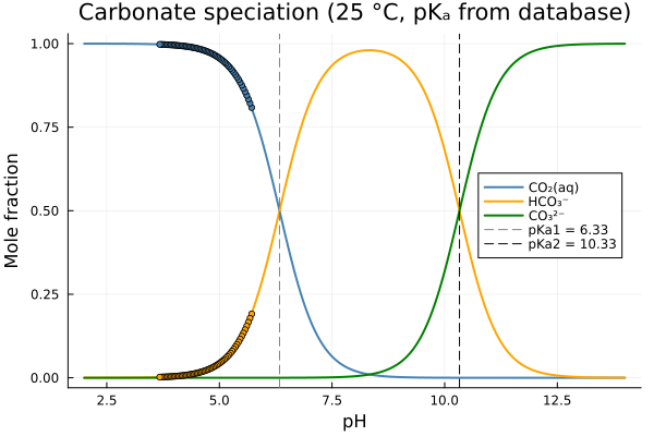

Analysis

Zone	pH range	Dominant species
Acidic / high CO₂	pH < 6.35 (pKₐ₁)	CO₂(aq)
Buffer zone 1	pH ≈ pKₐ₁ = 6.35	CO₂(aq) / HCO₃⁻ (equal amounts)
Mid-range	6.35 < pH < 10.33	HCO₃⁻
Buffer zone 2	pH ≈ pKₐ₂ = 10.33	HCO₃⁻ / CO₃²⁻ (equal amounts)
Alkaline	pH > 10.33	CO₃²⁻

Atmospheric CO₂ (~10⁻⁵ mol/L) produces a pH of ≈ 5.6 in pure water — slightly acidic rain even without any pollutants.
Carbonated water (industrial, ~0.05 mol/L CO₂) reaches pH ≈ 4.0–4.3.
Because dissolved CO₂ always pushes the system into the CO₂(aq)-dominated zone (pH < pKₐ₁), the HCO₃⁻ and CO₃²⁻ domains are only accessible by adding a base (e.g. NaOH, CaCO₃ dissolution) — which is the essence of ocean buffering and concrete alkalinity.

Link to cement chemistry

In the pore solution of hydrated cement (pH ≈ 12.5–13), the dominant carbonate species is CO₃²⁻. When atmospheric CO₂ penetrates the concrete cover, the carbonate system shifts leftward until portlandite (Ca(OH)₂) is consumed and the pH drops below 9. This process — carbonation — is the main cause of corrosion initiation in reinforced concrete, and is explored in the cement carbonation example.

CO₂ Dissolution and the Carbonate System ​

System setup ​

Dissociation constants from thermodynamic data ​

Building the equilibrium solver ​

CO₂ dissolution scan ​

Result: pH as a function of dissolved CO₂ ​

Speciation diagram ​

Analysis ​

CO₂ Dissolution and the Carbonate System

System setup

Dissociation constants from thermodynamic data

Building the equilibrium solver

CO₂ dissolution scan

Result: pH as a function of dissolved CO₂

Speciation diagram

Analysis