Getting started

Installation

To install ChemistryLab.jl, use the Julia package manager:

• From the Julia REPL, type ] to enter the Pkg REPL mode and run:

pkg> add ChemistryLab

• Or, equivalently, via the Pkg API:

julia> import Pkg; Pkg.add("ChemistryLab")

Citation

If you use ChemistryLab in your work, please cite the following:

@software{chemistrylab_jl,
  author       = {Barthélémy, Jean-François and
                  Soive, Anthony},
  title        = {ChemistryLab.jl: Numerical laboratory for
                   computational chemistry},
  doi          = {10.5281/zenodo.17756074},
  url          = {https://doi.org/10.5281/zenodo.17756074},
}

This quickstart shows a few common, minimal examples to get you productive with ChemistryLab. It demonstrates loading species from a database, building reactions and solving a thermodynamic equilibrium problem.

Simplified example

Let us start with a minimal example in which we compute the thermodynamic properties of a reaction. As a first illustration, we consider the equilibrium of calcite in water. This equilibrium can be written as:

It is possible to calculate the thermodynamic properties of the reaction, in particular the solubility constant of the reaction () which is related to the Gibbs free energy of the reaction (). This solubility constant is a function of temperature and the calculation is performed at a reference temperature of 298 K and at a pressure of 1 Atm using the following equation:

where is deduced from the Gibbs energies of formation () of the other chemical species involved in the reaction:

---

To do this, we load the species from one of the databases integrated into ChemistryLab, filter those relevant to the calcite–water system, then build the stoichiometric matrix and derive the reactions.

In this example, the database is cemdata. The .json file is included in ChemistryLab but is a copy of a file which can be found in ThermoHub.

build_species reads the database file and returns a Vector{Species} with compiled thermodynamic functions. speciation then filters this list to the species whose atomic composition is a subset of the seed atoms (here Ca, C, H and O from Cal, H2O@ and CO2):

using ChemistryLab
using DynamicQuantities # for unit management

all_species = build_species(datapath("cemdata18-thermofun.json"); verbose = false)
species_calcite = speciation(all_species, split("Cal H2O@ CO2");
                             aggregate_state=[AS_AQUEOUS],
                             exclude_species=split("H2@ O2@ CH4@"))
dict_species_calcite = Dict(symbol(s) => s for s in species_calcite)

Dict{String, Species{Int64}} with 12 entries:
  "Ca(HCO3)+" => Ca(HCO3)+ {CaHCO3+} [Ca(HCO3)+ ◆ Ca(HCO₃)⁺]
  "CaOH+"     => CaOH+ {CaOH+} [Ca(OH)+ ◆ Ca(OH)⁺]
  "HCO3-"     => HCO3- {HCO3-} [HCO3- ◆ HCO₃⁻]
  "H+"        => H+ {H+} [H+ ◆ H⁺]
  "CO2@"      => CO2@ {CO2  aq} [CO2@ ◆ CO₂@]
  "Ca(CO3)@"  => Ca(CO3)@ {CaCO3  aq} [CaCO3@ ◆ CaCO₃@]
  "CO3-2"     => CO3-2 {CO3-2} [CO3-2 ◆ CO₃²⁻]
  "CO2"       => CO2 {CO2  g} [CO2 ◆ CO₂]
  "Cal"       => Cal {Calcite} [CaCO3 ◆ CaCO₃]
  "Ca+2"      => Ca+2 {Ca+2} [Ca+2 ◆ Ca²⁺]
  "OH-"       => OH- {OH-} [OH- ◆ OH⁻]
  "H2O@"      => H2O@ {H2O  l} [H2O@ ◆ H₂O@]

During species creation, ChemistryLab calculates the molar mass of the species. It also constructs thermodynamic functions (heat capacity, entropy, enthalpy, and Gibbs free energy of formation) as a function of temperature. The evolution of thermodynamic properties as a function of temperature, such as heat capacity, can thus be easily plotted.

dict_species_calcite["Cal"]

Species{Int64}
           name: Calcite
         symbol: Cal
        formula: CaCO3 ◆ CaCO₃
          atoms: Ca => 1, C => 1, O => 3
         charge: 0
aggregate_state: AS_CRYSTAL
          class: SC_COMPONENT
     properties: M = 0.10008599996541243 kg mol⁻¹
                 Tref = 298.15 K
                 Pref = 100000.0 m⁻¹ kg s⁻²
                 Cp⁰ = 104.5163192749 + 0.02192415855825T + -2.59408e6 / (T^2) [m² kg s⁻² K⁻¹ mol⁻¹] ◆ vars=(T) ◆ T=298.15 K
                 ΔₐH⁰ = -1.2482415842895252e6 + 104.5163192749T + 2.59408e6 / T + 0.010962079279125(T^2) [m² kg s⁻² mol⁻¹] ◆ vars=(T) ◆ T=298.15 K
                 S⁰ = -523.9438829693111 + 0.02192415855825T + 104.5163192749log(T) + 1.29704e6 / (T^2) [m² kg s⁻² K⁻¹ mol⁻¹] ◆ vars=(T) ◆ T=298.15 K
                 ΔₐG⁰ = -1.1423813547027335e6 + 628.460202244211T + 1.29704e6 / T - 0.010962079279125(T^2) - 104.5163192749T*log(T) [m² kg s⁻² mol⁻¹] ◆ vars=(T) ◆ T=298.15 K
                 V⁰ = 3.6933999061584004e-5 [m³ mol⁻¹]
                 Cp⁰_Tref = 81.87109375 m² kg s⁻² K⁻¹ mol⁻¹
                 ΔₐH⁰_Tref = -1.207405e6 m² kg s⁻² mol⁻¹
                 S⁰_Tref = 92.675598144531 m² kg s⁻² K⁻¹ mol⁻¹
                 ΔₐG⁰_Tref = -1.129176e6 m² kg s⁻² mol⁻¹
                 V⁰_Tref = 3.6933999061584004e-5 m³ mol⁻¹

using Plots

p1 = plot(xlabel="Temperature [°C]", ylabel="Cp⁰ [J/mol/K]", title="Heat capacity of calcite \nas a function of temperature")
plot!(p1, θ -> dict_species_calcite["Cal"].Cp⁰(T = θ*ua"degC"), 0:0.1:100, label="Cp⁰")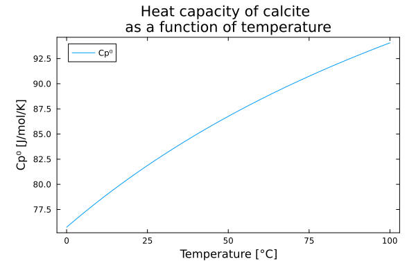

Obtaining stoichiometric matrices requires the choice of a species-independent basis.

primaries = [dict_species_calcite[s] for s in split("H2O@ H+ CO3-2 Ca+2")]
SM = StoichMatrix(collect(values(dict_species_calcite)), primaries)
pprint(SM)

┌───────┬───────────┬───────┬───────┬────┬──────┬──────────┬───────┬─────┬─────┬──────┬─────┬──────┐
│       │ Ca(HCO3)+ │ CaOH+ │ HCO3- │ H+ │ CO2@ │ Ca(CO3)@ │ CO3-2 │ CO2 │ Cal │ Ca+2 │ OH- │ H2O@ │
├───────┼───────────┼───────┼───────┼────┼──────┼──────────┼───────┼─────┼─────┼──────┼─────┼──────┤
│  H2O@ │           │     1 │       │    │   -1 │          │       │  -1 │     │      │   1 │    1 │
│    H+ │         1 │    -1 │     1 │  1 │    2 │          │       │   2 │     │      │  -1 │      │
│ CO3-2 │         1 │       │     1 │    │    1 │        1 │     1 │   1 │   1 │      │     │      │
│  Ca+2 │         1 │     1 │       │    │      │        1 │       │     │   1 │    1 │     │      │
└───────┴───────────┴───────┴───────┴────┴──────┴──────────┴───────┴─────┴─────┴──────┴─────┴──────┘

These stoichiometric matrices thus allow us to write the chemical reactions at work.

list_reactions = reactions(SM)
dict_reactions_calcite = Dict(r.symbol => r for r in list_reactions)

Dict{String, Reaction{Species{Int64}, Int64, Species{Int64}, Int64, Int64}} with 8 entries:
  "Ca(HCO3)+" => H⁺ + CO₃²⁻ + Ca²⁺ = Ca(HCO₃)⁺
  "Cal"       => CO₃²⁻ + Ca²⁺ = CaCO₃
  "CO2@"      => 2H⁺ + CO₃²⁻ = CO₂@ + H₂O@
  "CaOH+"     => H₂O@ + Ca²⁺ = Ca(OH)⁺ + H⁺
  "OH-"       => H₂O@ = OH⁻ + H⁺
  "HCO3-"     => H⁺ + CO₃²⁻ = HCO₃⁻
  "Ca(CO3)@"  => CO₃²⁻ + Ca²⁺ = CaCO₃@
  "CO2"       => 2H⁺ + CO₃²⁻ = CO₂ + H₂O@

Again, when constructing the reactions, the thermodynamic properties of the reactions as a function of temperature are deduced. It is thus possible to see, for example, the expression for the solubility product of calcite for the reaction under study and to plot its evolution.

dict_reactions_calcite["Cal"].logK⁰

NumericFunc:
  Unit: [m² kg s⁻² mol⁻¹]
  Variables: T, P
  References: T=298.15 K, P=100000.0 m⁻¹ kg s⁻²

p2 = plot(xlabel="Temperature [°C]", ylabel="pKs", title="Solubility product (pKs) of calcite \nas a function of temperature")
plot!(p2, θ -> dict_reactions_calcite["Cal"].logK⁰(T = θ*ua"degC"), 0:0.1:100, label="pKs")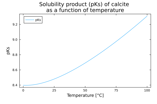

Equilibrium solving

The previous section computed thermodynamic properties of reactions analytically. ChemistryLab can go further and solve the full thermodynamic equilibrium — that is, find the species amounts that minimize the Gibbs free energy of the system given initial conditions.

Three objects are needed:

Object	Role
ChemicalSystem	Immutable description of the system: species list, primary species, stoichiometric matrices, and derived index maps. Built once and reused.
ChemicalState	Mutable thermodynamic state: amounts n (mol), temperature T and pressure P. Modified in-place before and after solving.
equilibrate	Convenience function that wraps a ChemicalSystem + ChemicalState into an optimization problem and solves it. Returns a new equilibrated ChemicalState.

using Optimization, OptimizationIpopt
using DynamicQuantities

# ChemicalSystem: declare the species and which four are the independent basis
primaries_eq = [dict_species_calcite[s] for s in split("H2O@ H+ CO3-2 Ca+2")]
cs = ChemicalSystem(collect(values(dict_species_calcite)), primaries_eq)

# ChemicalState: set the initial amounts
state = ChemicalState(cs)
set_quantity!(state, "Cal",  1e-3u"mol")   # 1 mmol of calcite
set_quantity!(state, "H2O@", 1.0u"kg")     # 1 kg of water

# Seed H⁺ and OH⁻ at pH 4 (trace amounts to help convergence)
V = volume(state)
set_quantity!(state, "H+",  1e-4u"mol/L" * V.liquid)
set_quantity!(state, "OH-", 1e-10u"mol/L" * V.liquid)

# Solve: find the Gibbs-energy minimum
state_eq = equilibrate(state)

┌ Warning: Verbosity toggle: missing_second_order_ad
│  The selected optimization algorithm requires second order derivatives, but `SecondOrder` ADtype was not provided. So a `SecondOrder` with AutoForwardDiff() for both inner and outer will be created, this can be suboptimal and not work in some cases so an explicit `SecondOrder` ADtype is recommended.
└ @ OptimizationBase ~/.julia/packages/OptimizationBase/TvAnm/src/cache.jl:116

The solved state in full — every species, with its amount

state_eq

ChemicalState{Species{Int64}, AbstractReaction, DynamicQuantities.Quantity{Float64, DynamicQuantities.SymbolicDimensions{DynamicQuantities.FRInt32}}, Float64}
┌─────────────────────────────────────────────────────────────────────────────────────────────────────────────────────┐
│           T : 298.15 K                                                                                              │
│           P : 1.0 bar                                                                                               │
╞═════════════════════════════════════════════════════════════════════════════════════════════════════════════════════╡
│  # liquid #│             n [mol]│               m [g]│             V [cm³]│           c [mol/L]│                    │
├┄┄┄┄┄┄┄┄┄┄┄┄┄┄┄┄┄┄┄┄┄┄┄┄┄┄┄┄┄┄┄┄┄┄┄┄┄┄┄┄┄┄┄┄┄┄┄┄┄┄┄┄┄┄┄┄┄┄┄┄┄┄┄┄┄┄┄┄┄┄┄┄┄┄┄┄┄┄┄┄┄┄┄┄┄┄┄┄┄┄┄┄┄┄┄┄┄┄┄┄┄┄┄┄┄┄┄┄┄┄┄┄┄┄┄┄┄┤
│ tot. liquid│             55.5096│             1000.02│             1002.96│                    │                    │
├┄┄┄┄┄┄┄┄┄┄┄┄┄┄┄┄┄┄┄┄┄┄┄┄┄┄┄┄┄┄┄┄┄┄┄┄┄┄┄┄┄┄┄┄┄┄┄┄┄┄┄┄┄┄┄┄┄┄┄┄┄┄┄┄┄┄┄┄┄┄┄┄┄┄┄┄┄┄┄┄┄┄┄┄┄┄┄┄┄┄┄┄┄┄┄┄┄┄┄┄┄┄┄┄┄┄┄┄┄┄┄┄┄┄┄┄┄┤
│        H2O@│             55.5093│             999.999│             1002.96│             55.3453│                    │
│        Ca+2│         0.000155243│          0.00622182│         -0.00286248│         0.000154784│                    │
│       HCO3-│         0.000133909│          0.00817059│          0.00324205│         0.000133513│                    │
│         OH-│          3.39679e-5│         0.000577693│        -0.000159916│          3.38676e-5│                    │
│       CO3-2│          2.13327e-5│          0.00128013│        -0.000129227│          2.12696e-5│                    │
│    Ca(CO3)@│          5.54915e-6│         0.000555392│         -8.68355e-5│          5.53275e-6│                    │
│   Ca(HCO3)+│          2.65111e-7│          2.68011e-5│          3.53387e-6│          2.64327e-7│                    │
│        CO2@│          8.86588e-8│          3.90179e-6│           2.9086e-6│          8.83969e-8│                    │
│       CaOH+│           8.7515e-8│          4.99579e-6│          5.04303e-7│          8.72564e-8│                    │
│          H+│         2.94308e-10│         2.96663e-10│                 0.0│         2.93439e-10│                    │
╞═════════════════════════════════════════════════════════════════════════════════════════════════════════════════════╡
│   # solid #│             n [mol]│               m [g]│             V [cm³]│                    │                    │
├┄┄┄┄┄┄┄┄┄┄┄┄┄┄┄┄┄┄┄┄┄┄┄┄┄┄┄┄┄┄┄┄┄┄┄┄┄┄┄┄┄┄┄┄┄┄┄┄┄┄┄┄┄┄┄┄┄┄┄┄┄┄┄┄┄┄┄┄┄┄┄┄┄┄┄┄┄┄┄┄┄┄┄┄┄┄┄┄┄┄┄┄┄┄┄┄┄┄┄┄┄┄┄┄┄┄┄┄┄┄┄┄┄┄┄┄┄┤
│  tot. solid│         0.000838855│           0.0839577│           0.0309823│                    │                    │
├┄┄┄┄┄┄┄┄┄┄┄┄┄┄┄┄┄┄┄┄┄┄┄┄┄┄┄┄┄┄┄┄┄┄┄┄┄┄┄┄┄┄┄┄┄┄┄┄┄┄┄┄┄┄┄┄┄┄┄┄┄┄┄┄┄┄┄┄┄┄┄┄┄┄┄┄┄┄┄┄┄┄┄┄┄┄┄┄┄┄┄┄┄┄┄┄┄┄┄┄┄┄┄┄┄┄┄┄┄┄┄┄┄┄┄┄┄┤
│         Cal│         0.000838855│           0.0839577│           0.0309823│                    │                    │
╞═════════════════════════════════════════════════════════════════════════════════════════════════════════════════════╡
│     # gas #│             n [mol]│               m [g]│             V [cm³]│                    │             p [bar]│
├┄┄┄┄┄┄┄┄┄┄┄┄┄┄┄┄┄┄┄┄┄┄┄┄┄┄┄┄┄┄┄┄┄┄┄┄┄┄┄┄┄┄┄┄┄┄┄┄┄┄┄┄┄┄┄┄┄┄┄┄┄┄┄┄┄┄┄┄┄┄┄┄┄┄┄┄┄┄┄┄┄┄┄┄┄┄┄┄┄┄┄┄┄┄┄┄┄┄┄┄┄┄┄┄┄┄┄┄┄┄┄┄┄┄┄┄┄┤
│    tot. gas│                 0.0│                 0.0│                 0.0│                    │                    │
├┄┄┄┄┄┄┄┄┄┄┄┄┄┄┄┄┄┄┄┄┄┄┄┄┄┄┄┄┄┄┄┄┄┄┄┄┄┄┄┄┄┄┄┄┄┄┄┄┄┄┄┄┄┄┄┄┄┄┄┄┄┄┄┄┄┄┄┄┄┄┄┄┄┄┄┄┄┄┄┄┄┄┄┄┄┄┄┄┄┄┄┄┄┄┄┄┄┄┄┄┄┄┄┄┄┄┄┄┄┄┄┄┄┄┄┄┄┤
│         CO2│                 0.0│                 0.0│                 0.0│                    │                 N/A│
╞═════════════════════════════════════════════════════════════════════════════════════════════════════════════════════╡
│   # TOTAL #│             n [mol]│               m [g]│             V [cm³]│                    │                    │
├┄┄┄┄┄┄┄┄┄┄┄┄┄┄┄┄┄┄┄┄┄┄┄┄┄┄┄┄┄┄┄┄┄┄┄┄┄┄┄┄┄┄┄┄┄┄┄┄┄┄┄┄┄┄┄┄┄┄┄┄┄┄┄┄┄┄┄┄┄┄┄┄┄┄┄┄┄┄┄┄┄┄┄┄┄┄┄┄┄┄┄┄┄┄┄┄┄┄┄┄┄┄┄┄┄┄┄┄┄┄┄┄┄┄┄┄┄┤
│            │             55.5105│              1000.1│             1002.99│                    │                    │
╞═════════════════════════════════════════════════════════════════════════════════════════════════════════════════════╡
│          pH : 9.5299                                                                                                │
│         pOH : 4.4702                                                                                                │
│    porosity : 0.999969                                                                                              │
│  saturation : 1.0                                                                                                   │
└─────────────────────────────────────────────────────────────────────────────────────────────────────────────────────┘

println("pH = ", round(pH(state_eq), digits = 2))

pH = 9.53

Derived quantities such as pH, pOH, phase volumes and individual species amounts are all accessible on the returned ChemicalState. For a detailed description of the solver options, activity models, and temperature sweeps, see the equilibrium tutorial (Tutorials → Chemical Equilibrium).

Notes and next steps

• The Formula, Species, Reaction and StoichMatrix APIs are intentionally small and composable — explore the docs/src/ pages for detailed examples.

• For equilibrium calculations, see docs/src/tutorials/equilibrium.md and the worked examples co2_carbonate_system and cement_carbonation.

• For cement-specific workflows, use CemSpecies and the databases utilities to convert between oxide- and atom-based representations.

Now try the quickstart examples interactively in the REPL and then follow the next pages of the tutorial for deeper coverage.

Quick tips

• In the REPL try small calls like using ChemistryLab; Species("CaCO3") and Formula("SO4-2") to explore parsing behavior interactively.

• Start with docs/src/examples/example_stoich_matrix.md to see a concise, runnable example converting a stoichiometric matrix into reactions.

• For equilibrium calculations, see docs/src/tutorials/equilibrium.md for the minimal workflow, then explore the co2_carbonate_system and cement_carbonation examples.

• If you plan to work with ThermoFun/Cemdata sources, run the examples in docs/src/tutorials/databases.md after placing the required .json/.dat data files in the data/ directory.

Next steps

You can see the examples section for more advanced runnable examples and small worked problems, including CO₂ dissolution, carbonate speciation, cement carbonation, and clinker dissolution.

Happy exploring — this tutorial aims to be practical and runnable, so please tell me which example you want expanded into a fully reproducible script.