Viscoelastic complex modulus of a bituminous mixture

The complex modulus of a bituminous mixture through three nested scales, following [88]. The bitumen is viscoelastic (2S2P1D); the mineral phases are elastic. Every scheme being ComplexF64-safe, the correspondence principle amounts to running the homogenization with complex-valued stiffnesses.

Scale	RVE	Phases	Scheme
1	Mastic	bitumen matrix + fillers	Mori-Tanaka
2	Mortar	mastic matrix + sand	Mori-Tanaka
3	Full mix	mortar matrix + coated coarse aggregates + pores	Self-Consistent

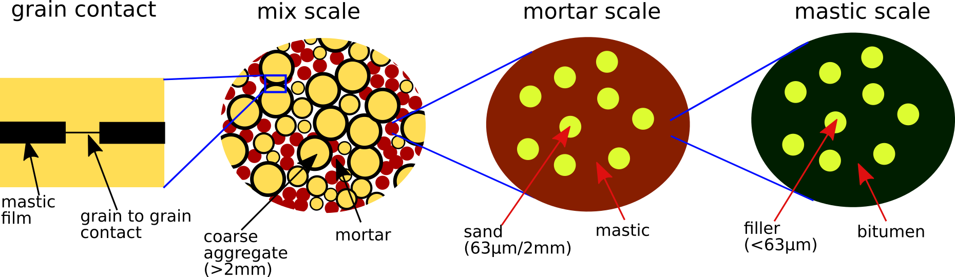
The coarse aggregates are coated grains — a stiff core wrapped in a thin mastic film — represented by a two-layer LayeredSphere that enters the self-consistent scheme through its concentration tensors (the composite-sphere support introduced for the cement-paste chapters, here with complex moduli).

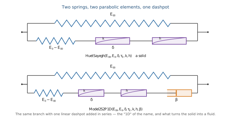
2S2P1D binder model

The bitumen complex Young's modulus in the Laplace-Carson domain ( ):

with the static modulus and the glassy one. This is Model2S2P1D from the rheological model library — the page used to define its own struct, and no longer needs to.

The parameter sets are unchanged

The inline struct this page carried named its fields the other way round (E0 for the static modulus, Einf for the glassy one), but its formula and its positional order were already the literature's. Switching to Model2S2P1D is therefore a pure rename: every one of the twelve calibrated sets below is copied argument for argument, and every number on this page is bit-identical to what it was.

One consequence worth having: E00 = 1e-7 was a numerical device to keep away from zero. A genuinely fluid binder, E00 = 0, is now legitimate — the fluid branch is handled exactly by kelvin_to_maxwell.

using MeanFieldHomogenization
using TensND
using LinearAlgebra
using Plots
gr()  # headless backend; GKSwstype is set to "100" in make.jl

# Hot-mix asphalt (HMA) — binders and experimental mix curves, ageing H0/H3/H9
E_BH0 = Model2S2P1D(1e-7, 1000.0, 2.2, 1.94507827e-3, 0.22, 0.63, 50.0)
E_BH3 = Model2S2P1D(1e-7, 1000.0, 2.12, 2.88910275e-3, 0.22, 0.611998586, 146.0)
E_BH9 = Model2S2P1D(1e-7, 1000.0, 2.85, 7.07911122e-3, 0.22, 0.61430255, 178.0)
E_EH0 = Model2S2P1D(86.3470095, 26000.0, 2.52254414, 0.834764484, 0.22, 0.65, 43.3031679)
E_EH3 = Model2S2P1D(20.0, 24362.0, 2.6, 2.6604, 0.199, 0.65, 900.0)
E_EH9 = Model2S2P1D(20.0, 24470.541, 2.73135009, 4.95748334, 0.175991713, 0.60, 900.0)

# Warm-mix asphalt (WMA) — binders and experimental mix curves, ageing W0/W3/W6
E_BW0 = Model2S2P1D(1e-7, 1000.0, 3.12, 9.49532017e-3, 0.22, 0.608684147, 101.0)
E_BW3 = Model2S2P1D(6.81e-6, 1000.0, 4.2, 3.209694e-2, 0.22, 0.55078753664, 393.0)
E_BW6 = Model2S2P1D(2.1e-4, 1000.0, 4.6, 3.78112337e-1, 0.22, 0.555320631, 808.0)
E_EW0 = Model2S2P1D(100.0, 21071.0, 2.4, 0.95, 0.207, 0.62, 9.45)
E_EW3 = Model2S2P1D(57.0, 20974.0, 2.6, 7.3168, 0.199, 0.59, 900.0)
E_EW6 = Model2S2P1D(100.0, 22290.0, 2.6, 89.095, 0.199, 0.59, 900.0)

Composition and volume fractions

The mix formula (mass fractions of the granular skeleton, bitumen mass fraction, and air voids) is converted to volume fractions through the phase densities.

compo_agg = Dict("6/10" => 0.2752, "4/6" => 0.1617, "2/4" => 0.1474,
    "sand" => 0.32285, "fines" => 0.0872)
size_agg = Dict("6/10" => 8.15, "4/6" => 5.15, "2/4" => 3.0)   # mean diameter (mm)

fmas = Dict{String,Float64}("bitume" => 0.054)
fvol0 = Dict{String,Float64}("pore" => 0.06)
ρ = Dict{String,Float64}(a => 2670.0 for a in keys(compo_agg))
ρ["bitume"] = 1040.0
for a in keys(compo_agg)
    fmas[a] = (1 - fmas["bitume"]) * compo_agg[a]
end
vtot = sum(fmas[a] / ρ[a] for a in keys(fmas))
for a in keys(fmas)
    fvol0[a] = (1 - fvol0["pore"]) * fmas[a] / ρ[a] / vtot
end
Dict(a => round(f, digits = 4) for (a, f) in fvol0)

Dict{String, Float64} with 7 entries:
  "pore"   => 0.06
  "sand"   => 0.266
  "fines"  => 0.0718
  "bitume" => 0.1207
  "2/4"    => 0.1214
  "6/10"   => 0.2267
  "4/6"    => 0.1332

Three-scale complex homogenization

The contact parameters set the mastic-film thickness (Duriez law), the mixing between pure mastic and a contact-stiffened film, and the film out-of-plane stiffness. Given a binder model, the function returns  . The coated aggregates are the complex two-layer LayeredSphere; the mix is closed with the self-consistent scheme.

const mod_agg, nu_agg, β0 = 9.5e4, 0.17, 0.51
const un = 1.0 + 0.0im

function Ehom(X, E_b)
    α, χ, kt = X
    Cagg = un * iso_stiffness_E_nu(mod_agg, nu_agg)
    fl = copy(fvol0)
    fmastic = fl["bitume"] + fl["fines"]
    e_film = Dict(a => α * 61.3e-3 * (size_agg[a] * 0.5)^β0 for a in keys(size_agg))
    ffilm = sum(fl[a] * ((1 + e_film[a] / (size_agg[a] * 0.5))^3 - 1) for a in keys(size_agg))
    fl["mastic_rest"] = fmastic - ffilm
    for a in keys(size_agg)
        fl[a] *= (1 + e_film[a] / (size_agg[a] * 0.5))^3
    end
    k_B = 2500.0
    μ_B(p) = 3k_B / (9k_B / carson_relaxation(E_b, p) - 1)

    function f(p)
        Cb = iso_stiffness(ComplexF64(k_B), μ_B(p))
        # Scale 1 — mastic (MT)
        fmastic_ = fl["bitume"] + fl["fines"]
        m = RVE()
        add_phase!(m, :bitume, Ellipsoid(1.0), Dict(:C => Cb); fraction = :rest)
        add_phase!(m, :fines, Ellipsoid(1.0), Dict(:C => Cagg); fraction = fl["fines"] / fmastic_)
        Cmastic = homogenize(m, MoriTanaka(), :C)
        # Scale 2 — mortar (MT)
        fmortar = fl["mastic_rest"] + fl["sand"]
        r = RVE()
        add_phase!(r, :mastic_rest, Ellipsoid(1.0), Dict(:C => Cmastic); fraction = :rest)
        add_phase!(r, :sand, Ellipsoid(1.0), Dict(:C => Cagg); fraction = fl["sand"] / fmortar)
        Cmortar = homogenize(r, MoriTanaka(), :C)
        # Scale 3 — full mix (SC) with coated aggregates
        v = RVE()
        add_phase!(v, :mortar, Ellipsoid(1.0), Dict(:C => Cmortar); fraction = :rest)
        for a in keys(size_agg)
            ka, _ = k_mu(Cagg)
            Cfilm = χ * Cmastic + (1 - χ) * iso_stiffness(ka, ComplexF64(e_film[a] * kt))
            ra = size_agg[a] * 0.5
            sphere = LayeredSphere((ra, ra + e_film[a]), (Cagg, Cfilm))
            add_phase!(v, Symbol(a), sphere, Dict(:C => Cagg); fraction = fl[a])
        end
        add_phase!(v, :pore, Ellipsoid(1.0), Dict(:C => un * TensISO{3}(0.0, 0.0));
            fraction = fl["pore"])
        return E_nu(homogenize(v, SelfConsistent(; abstol = 1e-10, maxiters = 100), :C))[1]
    end
    return f
end

The pre-calibrated contact parameters (from the COBYLA fit of the least-aged state in [73] — the calibration itself is not repeated here) are used directly. A check against the Echoes reference at four frequencies:

x_HMA = (5.866e-3, 0.9760, 6366.1)
Ef = Ehom(x_HMA, E_BH0)
for ω in (1e-3, 1e-1, 1e1, 1e2)
    z = Ef(im * ω)
    println("ω = ", rpad(ω, 7), "  |E*| = ", rpad(round(abs(z), digits = 1), 9),
        " MPa   δ = ", round(rad2deg(angle(z)), digits = 2), "°")
end

ω = 0.001    |E*| = 223.7     MPa   δ = 29.75°
ω = 0.1      |E*| = 3113.9    MPa   δ = 37.92°
ω = 10.0     |E*| = 9082.9    MPa   δ = 14.05°
ω = 100.0    |E*| = 12572.3   MPa   δ = 11.13°

These reproduce the Echoes values (|E*| ≈ 224 / 3114 / 9083 / 12572 MPa, δ ≈ 29.8 / 37.9 / 14.1 / 11.1°) to the SC convergence tolerance.

Contact-parameter calibration

The three contact parameters are calibrated by minimizing the relative distance between the multi-scale model and the experimental master curve of the least-aged state,

subject to inequality constraints keeping the fit acceptable for the more-aged states. [88] minimize it with a derivative-free COBYLA routine; their parameters are used directly here rather than re-calibrated:

x_HMA = (5.866e-3, 0.9760, 6366.1)   # J = 4.10e-1
x_WMA = (4.165e-2, 0.9791, 3277.7)   # J = 2.39e-1

Master curves: binder amplification across ageing states

For each ageing state the binder stiffness (dashed) is amplified by roughly three decades to the mix modulus (solid); the mix phase angle stays below the binder's, reflecting the stiffening by the rigid granular skeleton. Markers are the experimental 2S2P1D master curves. The same plot_mix helper is reused for the hot-mix (HMA) and warm-mix (WMA) asphalts.

ωs = 10.0 .^ range(-3.5, 2.5; length = 22)
cols = (:black, :red, :blue)

function plot_mix(x_opt, states, title)
    pE = plot(; xscale = :log10, yscale = :log10, xlabel = "ω (rad/s)",
        ylabel = "|E*| (MPa)", legend = :bottomright, framestyle = :box)
    pδ = plot(; xscale = :log10, xlabel = "ω (rad/s)", ylabel = "δ (°)",
        legend = false, framestyle = :box)
    for ((name, E_b, E_e), c) in zip(states, cols)
        Em = Ehom(x_opt, E_b)
        plot!(pE, ωs, [abs(complex_modulus(E_b, ω)) for ω in ωs]; ls = :dash, c = c, lw = 1.5, label = "binder $name")
        plot!(pE, ωs, [abs(Em(im * ω)) for ω in ωs]; c = c, lw = 2, label = "mix $name (model)")
        scatter!(pE, ωs, [abs(complex_modulus(E_e, ω)) for ω in ωs]; c = c, ms = 2.5, markerstrokewidth = 0, label = "")
        plot!(pδ, ωs, [rad2deg(angle(complex_modulus(E_b, ω))) for ω in ωs]; ls = :dash, c = c, lw = 1.5)
        plot!(pδ, ωs, [rad2deg(angle(Em(im * ω))) for ω in ωs]; c = c, lw = 2)
        scatter!(pδ, ωs, [rad2deg(angle(complex_modulus(E_e, ω))) for ω in ωs]; c = c, ms = 2.5, markerstrokewidth = 0)
    end
    return plot(pE, pδ; layout = (1, 2), left_margin = 8Plots.mm, bottom_margin = 8Plots.mm, size = (1000, 450), plot_title = title)
end

plot_mix(x_HMA, (("H0", E_BH0, E_EH0), ("H3", E_BH3, E_EH3), ("H9", E_BH9, E_EH9)),
    "Hot-mix asphalt (HMA) — model vs experiment")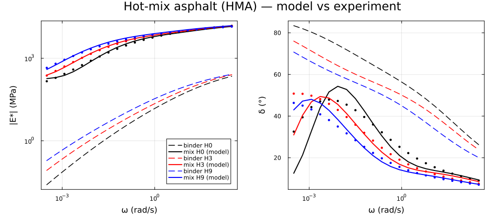

plot_mix(x_WMA, (("W0", E_BW0, E_EW0), ("W3", E_BW3, E_EW3), ("W6", E_BW6, E_EW6)),
    "Warm-mix asphalt (WMA) — model vs experiment")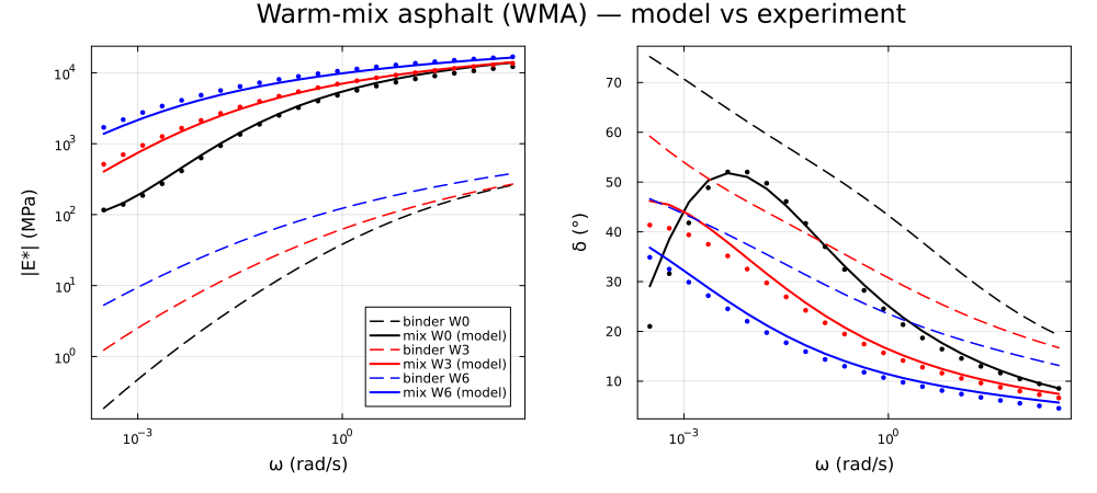

In both mixes the ageing states shift the master curve toward higher stiffness and lower phase angle as the binder hardens — the model tracks the experimental curves across the whole frequency range with a single calibrated parameter set per mix.

Back to the time domain

Everything above lives in the frequency domain, which is where the material is measured. A pavement, though, is loaded by a wheel passing over it — a transient, not a sinusoid — so what a structural calculation needs is the relaxation modulus .

That is one call. homogenize_lc takes the same three-scale cell builder used above, evaluates it at whatever Carson variables the inversion algorithm asks for, and returns the time-domain answer directly:

E_of_t(x_opt, E_b, times; method = FixedTalbot(24)) =
    inverse_carson(Ehom(x_opt, E_b), times, method)

t_grid = exp10.(range(-6, 4; length = 60))
E_H0 = E_of_t(x_HMA, E_BH0, t_grid)
E_H9 = E_of_t(x_HMA, E_BH9, t_grid)

pt = plot(
    t_grid, real.(E_H0);
    xscale = :log10, yscale = :log10, lw = 2.5, c = 1,
    xlabel = "t  (s)", ylabel = "E_hom(t)  (MPa)", label = "HMA, state H0",
    title = "Relaxation modulus of the mix", legend = :bottomleft,
)
plot!(pt, t_grid, real.(E_H9); lw = 2.5, c = 3, label = "HMA, state H9 (aged)")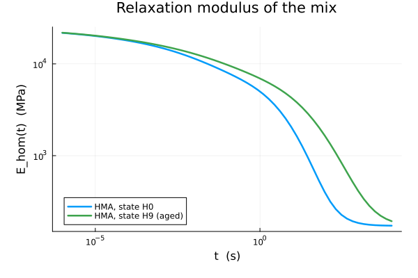

Note what is not here: no time grid was needed to get the value at  , no Volterra operator was assembled, and no time-marching took place. Each point costs 24 evaluations of the three-scale chain and nothing else — the transform carries the whole memory of the material.

The ageing states separate the same way they do on the master curve, only read from the other end: the aged binder gives a stiffer mix at every time, and the gap widens as the load becomes slower.

Which inversion, and why it matters here

Every point costs N full three-scale homogenizations — a self-consistent scheme nested inside two Mori-Tanaka estimates — so the choice is a real one:

• FixedTalbot(24), used above, is the most accurate;

• GaverStehfest(16) needs a third fewer evaluations and keeps them all at real p, so the whole chain runs in real rather than complex arithmetic. It costs about five significant digits, which is well inside the uncertainty on any calibrated binder;

• DeHoog shares one node set across a block of times, which pays off precisely on a ten-decade grid like this one.

See the inversion manual. The 2S2P1D transform has a branch cut at the origin, from its terms; that is not an obstacle for any of them — the Talbot contours are designed to wrap around exactly such a singularity.