Concave pores: superspheres and superspheroids

A supersphere

is the sphere at  , the octahedron at  , and below that a concave body with conical points on the three axes — a reasonable idealization of the pore shapes that scanning electron microscopy finds in sandstone and in harzburgite. It has no Eshelby solution, so it is exactly the morphology FESupershapePore exists for.

[85] studied it by finite elements and condensed the result into a single scalar — the only published data for this shape family, and what makes any comparison possible at all. This page reports what the package computes on the same shapes: the agreement is exact where the answer is known, and two quantities come out differently. One is the anisotropy, which their scalar summary does not set out to carry; the other is a fit in , read pointwise rather than over the range it summarizes. The numbers below are ours, and the published values are quoted as they stand.

This page is static

The figures and the numbers are produced once by scripts/fe/make_cell_figures.jl and committed; the live demonstration is scripts/89_fe_concave_pores.jl.

The cell, and why one eighth of it is enough

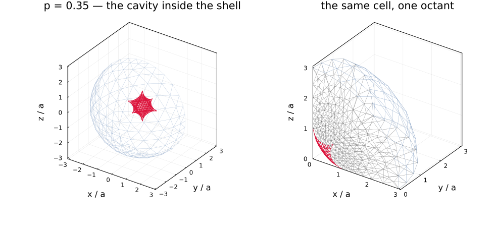
The three coordinate planes are mirror planes of a supersphere, so the cell is invariant under a group of order eight and an octant carries the whole answer — see the pore declination for the parity argument and for why the dipole correction survives it. That is not a convenience here, it is what makes the study possible: at   the whole cell needs some 360 000 degrees of freedom at level 4 and does not fit on a 16 GB machine, while the octant needs about 70 000 and takes half a minute.

The left panel is the whole cell of a concave shape at  , cut away so the cavity is visible; the right panel is the same cell as an eighth, with the three flat faces that had to be built in gray.

What can be checked exactly

Two of the three checks below are against their published work, and both pass; that is the headline of this section.

The volume, to machine precision. Their Eq. (2.7) and the closed form this package derives independently agree to   over the whole range, including the two values known exactly: at the sphere and at the octahedron.

The spherical limit. At   the measured resistivity contribution is   against the exact — a relative error of   at level 3, and   at level 4, which the octant makes affordable. This is the control for everything else on this page.

Their near the sphere. The fit is anchored at the sphere, where the answer is exact, so the two agree to   at   and to 2 % at  .

The scalar fit in , read pointwise

is a linear fit in , pinned at  , where it is exact, and at  , where the effect is taken to vanish. A straight line through two points is an economical summary, chosen for the use their paper makes of it; what follows compares it with the pointwise values computed here, which is a harsher test than it was designed for:

	here	their	difference
0.30	1.9288	3.4589	−44 %
0.40	1.6581	2.2392	−26 %
0.50	1.5763	1.7671	−11 %
0.70	1.5152	1.4853	+2.0 %
1.00	1.4998	1.5000	−0.013 %
1.50	1.5111	1.7923	−16 %
2.50	1.5400	2.6065	−41 %

The two convex rows lie outside the stated range of validity — the fit is restricted to   — so they are given for context only. Two further properties follow from pinning a straight line at  , and they are worth knowing before reusing the expression outside its intended role: read pointwise, is non-monotone near the lower anchor (zero at by construction, just above at ), and it changes sign below , so it should not be extrapolated there.

The cubic anisotropy, measured on its own three invariants

A supersphere is cubic, and two constants cannot express that. The octahedral group leaves three invariants for a fourth-order tensor with the minor symmetries, and below   the third is not a small correction. Eq. (2.19) writes the compliance contribution on the isotropic basis — two constants, an entirely usual way to condense such a result and enough for the scalar that paper sets out to report — and its Fig. 4 data is isotropic to about 1 % on the ratio across the whole range. So the third invariant is not a quantity to be compared: it is one the published study does not undertake to deliver, and one this package can add to it.

This package measures the three separately, because TensND.TensCubic is a storage class in its own right and the octant makes the cubic structure exact rather than approximate: the couplings symmetry forbids come out identically zero instead of as mesh noise at a few percent of the norm.

				anisotropy
0.30	3.3167	−0.7771	1.5680	+0.2888
0.40	2.5262	−0.6063	1.3265	+0.1899
0.50	2.2954	−0.5551	1.2566	+0.1470
0.70	2.0955	−0.5097	1.2289	+0.0703
1.00	2.0094	−0.4798	1.2444	+0.000246
1.50	1.9709	−0.4513	1.2828	−0.0728
2.50	1.9668	−0.4246	1.3426	−0.1493

"Anisotropy" is Zener's ratio   , identically zero for an isotropic tensor. Read the middle row first. At   the body is a sphere and the true anisotropy is zero, so   is this chain's own spurious anisotropy at this discretization — on the same mesh generator, element and quadrature as every other row. The concave signal is 1170 times larger than that, and the convex one 600 times. It also changes sign at the control, which no numerical artifact would do: a concave supersphere and a cube-like one are anisotropic in opposite senses.

The cost, and what the octant buys. Same spherical pore, same corrected condition, both modes:

level	mode	vector dofs	conduction error	time
2	whole	12 165	2.86e-3	8.5 s
2	octant	2 604	1.05e-3	0.1 s
3	whole	31 881	2.74e-4	0.4 s
3	octant	5 898	1.31e-4	0.0 s
4	octant	17 508	9.73e-6	0.2 s

The octant is not merely cheaper at equal level: it is about twice as accurate, because the parity projection removes couplings that the whole cell carries as noise. At   it also needs no snapping fallback where the whole cell backs off on 37 nodes.

What the paper allows us to conclude, and what it does not. Their values are published as figures rather than tables, on linear tetrahedra with a surface integral built from centroid values on flat triangles, so the anisotropy cannot be read back out of them to be compared component by component. What can be said is on the table above, and it concerns this chain alone: the control row bounds its own spurious anisotropy, and the measured signal is three orders of magnitude above it.

The axisymmetric companion, where the data is tabulated

[86] is the same team's study of the axisymmetric concave pore. Its shape, Eq. (1.2),

is Superspheroid(a, aγ, p) without conversion, studied at a = γ = 1. Being a solid of revolution it is transversely isotropic — five constants for ℍ, two for ℝ — and it is the only one of the two papers to tabulate its numbers, which makes a component-by-component comparison possible where Chen et al.'s figures allow only a comparison of trends.

Two conventions for p

On this page p is the concavity exponent of the shape, with 2p the exponent of the level set. It is not the confocal angular coordinate of the layered spheroid, nor the mode-1 nodal unknown of the axisymmetric solver. Coordinates here are cylindrical throughout, and the aspect ratio is written c/a.

It needs a different tool, and gets one

The fields separate into Fourier modes in the azimuth, so each mode is a two-dimensional problem on the meridian half-plane — the same reduction as for the recycled aggregate, and where the octant divides the three-dimensional cost by eight this divides it by orders of magnitude. FEAxiSupershapePore is that cell, and the mode count delivers exactly the five constants: a   block from mode 0, a scalar from mode 1, a scalar from mode 2.

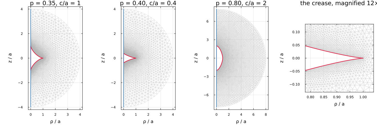
Being two-dimensional, that picture is the whole computational domain rather than a slice of one, which is the point of showing it. The cavity wall is in crimson, drawn from the closed-form profile and not from the mesh, and the revolution axis in blue; nothing is prescribed on the wall, and that is what makes it a cavity.

The fourth panel is the equatorial crease, magnified, and it is there because uniform elements are not enough. A concave superspheroid closes at the equator as a wedge: at    the half-gap is where a uniform element is , so elements straddled a gap twenty-five times thinner than themselves. The symptom was specific — mode 0's stopped converging while mode 1's converged cleanly — and the cure is to grade the element size in the distance to the two corners, for concave profiles only. That took the refinement increment from   to  , and the ungraded value was 1.2 % wrong rather than merely unconverged.

Whether some is simply too concave to mesh, needing extrapolation instead, was measured rather than assumed: the minimum mesh angle stays between 33.8° and 39.5° down to  , so there is no floor and no degenerate element.

Two of its numbers are statements rather than measurements, and they are what license reading the rest. Transverse isotropy holds to at any refinement, being structural rather than converged, which checks the three modes, the azimuthal projections, the boundary integral and the Kelvin reassembly simultaneously. And conduction on a sphere is exact to   and does not improve with refinement, a spherical cavity's exterior perturbation being a pure dipole with no higher multipole left to truncate.

The reference moduli, inferred

The paper reports dimensionless quantities and states no modulus, so one has to be recovered before the tables can be compared. What follows uses E₀ = 1, ν₀ = 1/3, k₀ = 1, inferred from its own p = 1 row: there the body is an exact sphere, Eq. (3.9) applies, and H₁₁₁₁/(−H₁₁₂₂) = (9+5ν₀)/(1+5ν₀) gives ν₀ = 0.330. With ν₀ = 1/3 all five components and both resistivities come back to 0.06 %, which is their own finite-element error. It is an inference and is presented as one.

The closed forms, and the conventions to read them with

Its tables are self-consistent, and it is the tables this page compares against. Reproducing the printed closed forms literally does not return those tables, so four readings have to be adopted for the two to agree; each is checked on the p = 1 row, where the answer is known independently. They are recorded here to save the next reader the same detective work, not as a criticism of a paper whose data is sound.

1. V*(p) in Eqs. (3.10)–(3.11) is to be read as the normalized volume 3g(p) = V*/(4π/3), not as the volume of Eq. (1.3). Read as the volume itself, H₃₃₃₃(p=1) comes out 0.477 instead of 2.001 — a factor 4π/3.

2. A factor of four on the shear components. Evaluated as printed, H₁₃₁₃ and H₁₂₁₂ from Eq. (3.5) give 5.0 for the sphere where 1.25 is expected.

3. A sign. Eq. (3.5) reads H₁₂₁₂ ≡ (H₁₁₁₁ + H₁₁₂₂)/2; the difference is what matches the tables. On their own Table B.1 at p = 1, the minus gives 1.2496 and the plus 0.7516.

4. Eq. (3.10) appears to mix the two shear conventions, H₁₂₁₂ being written in the tensor one and H₁₃₁₃ in the other.

None of this affects the tabulated values, which is why the tables are what this page compares against and the closed forms are not.

The two tables, superimposed

All eighteen rows of their Table B.1 and all seventeen of their Table B.4, plotted as points against this package's Fourier cell as a line. Both are dimensionless in the form the paper reports them: for the compliance contribution and for the resistivity, with    under the inference above, so the plotted numbers are the tabulated ones. The panel axes carry those factors; the prose below writes and plainly, this convention being stated once here.

The last panel is the comparison itself — every deviation on one logarithmic axis — and the only place their Table B.3 appears: the largest relative change between their two meshes at each , plotted as its own curve. That is their own published estimate of their resolution, and it is the fairest yardstick a deviation can be read against; nothing is drawn on their tabulated values that they did not put there.

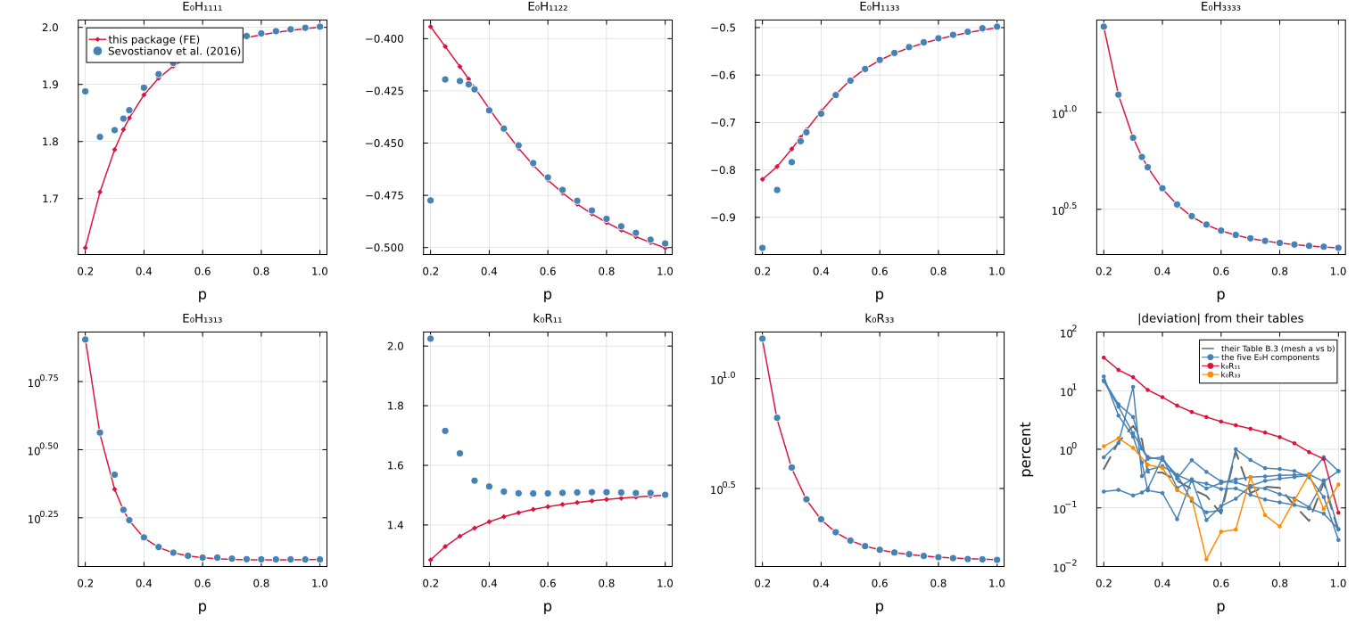
Four of the five compliance components, and the axial resistivity, agree across the whole range. is the demanding one — it runs from 2.00 at the sphere to 27.7 at  , a factor of fourteen — and it agrees to 0.72 % or better everywhere, 0.19 % at the most concave row. agrees to 1.6 %, to 0.5 % except at two rows discussed below, and for   the transverse block agrees to 0.75 %, which is at or below the change between their own two meshes.

That is the agreement, and it is worth stating plainly before the disagreements: two independent finite-element formulations — theirs three-dimensional on a million-node mesh, ours two-dimensional on sixty thousand — land on the same five-constant tensor over a shape family with no closed form.

Three differences, of three different kinds

One is a trend, not an amplitude. Their rises with concavity — 1.5012 at the sphere, 1.6400 at  , 2.0247 at   — where ours falls: 1.5000, 1.3624, 1.2830. At the most concave row that is a deviation of 37 %, and no refinement of ours closes it. That was checked before it was written: across radius_ratio from 4 to 10 — a factor 2.5 on the cell radius — and nradial from 20 to 28, at   is 1.28298 in all eight configurations, unchanged to six figures, with stable to and to  .

Before anything else: the two computations are solving the same body. Their Table C.1 gives the dimensionless volume in closed form at four values, and the package's own closed form matches all four to machine precision — at  , at , at , at the sphere, residuals below  . Whatever the difference is, it is not a difference of geometry.

Nor can it be a matter of normalization. and are normalized by the same cavity volume, so an error there would move every component by one common factor — and and agree with their tables to 0.7 % and 1.6 %. A factor that leaves those alone while moving by 37 % does not exist.

The physics does not settle this by inspection, which is worth saying rather than glossing. As   with   the body tends to an equatorial disc pierced by a needle along . Under a transverse gradient a disc in its own plane is transparent and contributes 1, while a needle parallel to is a two-dimensional obstacle and contributes 2. Our 1.28 and their 2.02 sit either side of that pair, so the question is which of the two features carries the limit — not which curve is obviously wrong.

One reference point is available to both: at   the body is an exact sphere, where  . We obtain 1.500000 and their table gives 1.501244, i.e. within 0.08 % of the exact value — consistent with the finite-element resolution their own Table B.3 reports, and far too small to account for the 37 %.

What does bear on the question is that the package can solve the same shape twice, by two routes with nothing in common: the Fourier cell on a meridian mesh, and the three-dimensional octant cell of the supersphere section, on tetrahedra. At  :

Fourier axisymmetric, 2-D	1.78579	7.39345	1.36238	3.89764
octant, 3-D, level 3	1.76599	6.81044	1.35528	3.62208
octant, 3-D, level 4	1.78023	7.07750	1.36066	3.74200
[86]	1.81996	7.40550	1.64000	3.93922

The octant gives  , 0.13 % from the two-dimensional value and rising towards it as the level increases. Two independent discretizations of ours meet, and the tabulated value sits 17 % from both. The octant is not a variant of the Fourier cell: different mesher, different elements, different assembly, and no azimuthal modes anywhere — so a fault in the mode-1 transport operator, the one place a -only error could hide, would have to be reproduced by a code that has no modes. That same operator is what the exact oblate and prolate spheroid gates exercise, since   there and both are closed-form.

The transverse resistivity, and what we make of it

Their column has a property worth noting: over   it is flat to 0.3 % — 1.5055, 1.5059, 1.5075, 1.5091, 1.5099, 1.5099, 1.5089, 1.5070, 1.5073 — while over the very same rows their own falls by 14 % and their by 22 %. It also sits above their sphere value throughout, and wiggles non-monotonically inside that band. Ours rises smoothly over the same interval, 1.452 to 1.497, and lands on 1.500000 at the sphere.

We have no established explanation for the difference. The most economical one we can think of is that the transverse resistivity is the most demanding of the seven quantities for a three-dimensional mesh, so it is where two discretizations would be expected to part company first — but that is a conjecture, not a result, and nothing here proves that our value is the converged one either. What would settle the question is a third, independent implementation, and none is published for this shape family, which is precisely what makes their study valuable.

The same table carries its own counter-check, and that one runs in their favor. On their 7.4055 is 0.16 % from our two-dimensional value, while our own octant at level 4 gives 7.0775 — 4 % below, and still climbing. Three-dimensional meshes converge slowly from below on that component: their million-node mesh has got there and our level 4 has not, which is a point in favor of their discretization. It is also consistent with the transverse block being the harder part of the problem for a three-dimensional mesh, and with the reversal appearing exactly at  .

One is a change of direction in the transverse block. Below   the tabulated values reverse: is 1.8878 at  , falls to 1.8080 at  , then rises again to 1.8200 at  , and and do the same. Ours is monotone throughout. The deviation reaches 14.5 %, 17.4 % and 15.0 % at  , and it appears exactly where a three-dimensional mesh has to resolve six conical points that a meridian mesh sees as two corners on a curve — which is a difference of method before it is a difference of result.

And one row is not usable for comparison. is listed as 1.269780 at   and again, to six decimals, at  ; we set that row aside rather than read a deviation from it. Table B.3 marks the same row with 0.91 %, the largest change in that column, and  , where the two differ by 11.6 %, carries its second largest at 0.83 % — their own mesh study had already identified both as the least settled, which is exactly the information one needs to read a comparison honestly.

One limitation, and it belongs to one of the two families

The three-dimensional cell. In the concave range the measured tensor departs from cubic symmetry by about , and that does not improve with refinement:   at level 4 against   at level 3. What limits it is the singular field at the conical points, not the mesh density — the same mechanism that makes the boundary snapping back off there. It is the accuracy the teacher has, and it sets the tolerance of the supersphere surrogate's training set.

The axisymmetric cell has no such limit, transverse isotropy there being structural rather than converged, so its residual is round-off at any refinement. Its own accuracy is bounded by the cell radius instead — truncation, which the dipole correction reduces from to but does not abolish — and by the fit of the two surrogates trained on it, which is where the graded mesh and the geometric sampling above were spent.

Reproducing this page

julia scripts/fe/make_cell_figures.jl        # figures + docs/src/assets/fe/cell_results.md.in
julia scripts/89_fe_concave_pores.jl      # the comparison, live

See also

• The finite Eshelby cell with a corrected boundary condition — the pore declination, and the octant's parity argument.

• Finite-element inclusions — how to use the type.

• Neural-surrogate inclusions — the trained models that replace the solve.

References

1. F. Chen, I. Sevostianov, A. Giraud and D. Grgic. Evaluation of the effective elastic and conductive properties of a material containing concave pores. International Journal of Engineering Science 97, 60–68 (2015).

2. I. Sevostianov, F. Chen, A. Giraud and D. Grgic. Compliance and resistivity contribution tensors of axisymmetric concave pores. International Journal of Engineering Science 101, 14–28 (2016).