A recycled-concrete aggregate, by axisymmetric Fourier elements

Recycling concrete means crushing it, and what comes out is not a clean aggregate: each grain is an old natural aggregate wrapped in a shell of adhered old mortar, of uncertain and generally poor quality, and the old aggregate is not centered in its shell. [68] homogenized that morphology by generalizing the Eshelby problem to an inclusion of arbitrary internal structure, solved by finite elements. This page reproduces their study with FEExcenteredSphere, and improves on it in one respect.

The paper solves the cell in full three dimensions. The morphology is a solid of revolution, though, so the fields can be expanded in Fourier series in the azimuth and each mode solved on the meridian half-plane. Four two-dimensional problems replace six three-dimensional ones and the cost drops by two orders of magnitude at equal accuracy — a first evaluation takes two seconds. The boundary condition is the same first-order corrected one as for the elliptical crack, here in its general form, with the polarization fixed point rather than the crack's 3 + 3 shortcut.

Nothing downstream knows any of this: the inclusion satisfies the custom-inclusion contract and every scheme takes it.

This page is static

Every figure and number below was produced once by scripts/fe/make_axi_figures.jl and committed. Nothing here runs at documentation-build time, so building the docs needs neither gmsh_jll nor a single finite-element solve.

The morphology

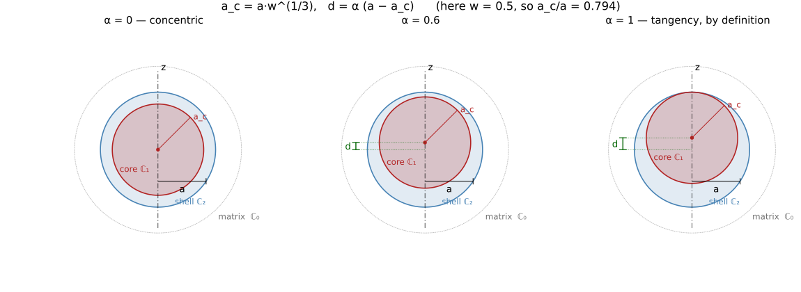
Meridian section, drawn at   (hence  ), the value used throughout this page. Left to right: the concentric limit, an intermediate eccentricity, and the tangency limit that defines the normalization of .

Symbol	Meaning
	radius of the whole inclusion (a, the first constructor argument)
	volume fraction of the core inside the inclusion (core_fraction)
	core radius, fixed by
	offset of the core center along the symmetry axis
	eccentricity (eccentricity): the offset as a fraction of the largest one the geometry admits
	radius of the surrounding ball of matrix (radius_ratio, in units of )
	stiffness of the core and of the shell (props, in that order)
	stiffness of the reference medium, the fresh paste

The normalization is what makes readable:   is the distance the core center can travel before the core touches the outer surface, so runs over whatever is, and   is tangency by construction. Values above 1 are geometrically impossible and rejected.

  is the concentric two-layer sphere, for which LayeredSphere gives the exact Hervé-Zaoui answer — the reference everything below is checked against. The response is transversely isotropic about , and isotropic at  .

Fourier expansion in the azimuth

Write cylindrical coordinates with the symmetry axis. In elasticity the Fourier mode is

and in transport  . The cylindrical strain components follow:

the first column carrying and the second .

Why the modes do not couple. The elastic energy is       . A material transversely isotropic about the axis has no coupling between the group and the group, so the only azimuthal integrals left are   and   — both equal to for  , and for the group at  . Different modes meet only through  , which vanishes. Each mode is therefore an independent two-dimensional problem, and the leftover constant multiplies the whole quadratic form — irrelevant here, since the right-hand side is a pure Dirichlet lift.

Which mode a loading excites. A constant macroscopic strain decomposes on the Kelvin basis adapted to the axis, and each basis tensor lives in exactly one mode:

Macroscopic loading	Boundary displacement	Mode
		0
		0
		1
		2
		0
		1

Four elastic loadings, not six: the partners     and     are obtained by rotating about the axis and share the eigenvalue of their mode. Six Kelvin coordinates, six independent components — exactly the dimension of a transversely isotropic fourth-order tensor without major symmetry, which is what a localization tensor is.

The axis

  is a boundary of the computational domain without being a boundary of the body. Single-valuedness of the three-dimensional field there forces

and in transport   for  , nothing for  .

The   condition couples two components, which a plain Dirichlet condition cannot express. Rather than reach for an affine constraint, the code changes unknowns:

after which the conditions read   and   — two ordinary Dirichlet conditions. The substitution earns a second dividend: in the strain operator every term is then attached to a constrained unknown ( ,     ,     ), so the singular integrands vanish where they would otherwise be sampled.

Averaging back to Cartesian

The scheme needs and as Cartesian tensors. The azimuthal integration is done analytically. With the modal amplitude of a symmetric second-order field,

and in transport    for  ,     for  . What remains is the meridian quadrature with the measure   , and the volume    .

Projecting on the Kelvin basis of the mode turns those averages directly into the modal blocks of and , and the blocks reassemble into the   Kelvin matrix of a transversely isotropic tensor.

The corrected boundary condition

The truncated cell is the same problem as for the crack, and has the same answer: the polarization fixed point of The finite Eshelby cell. Only one thing is specific here — each fixed point lives inside one Fourier mode, since the dipole of a modal polarization radiates in the same mode, so is   for mode 0 and a scalar for modes 1 and 2.

The two dipole fields are resolved on the cylindrical basis mode by mode. Each branch vanishes on the axis exactly where the modal axis conditions require it, so the outer and the axis conditions never contradict each other at the poles — a small thing, but it is what lets the two prescribed sets be merged without arbitration.

What is solved

Physics	Modes	Assemblies	Solves
elasticity	0 (2 dofs/node), 1, 2 (3 dofs/node)	3	8 = 4 affine + 4 dipole
transport	0, 1 (1 dof/node)	2	4 = 2 affine + 2 dipole

Each mode is assembled once and factorized once; both right-hand-side families reuse that factorization. Straight triangles carry a P1 or P2 field (order); the quadrature is of order   , one degree above the material term, to absorb the weight.

The mesh

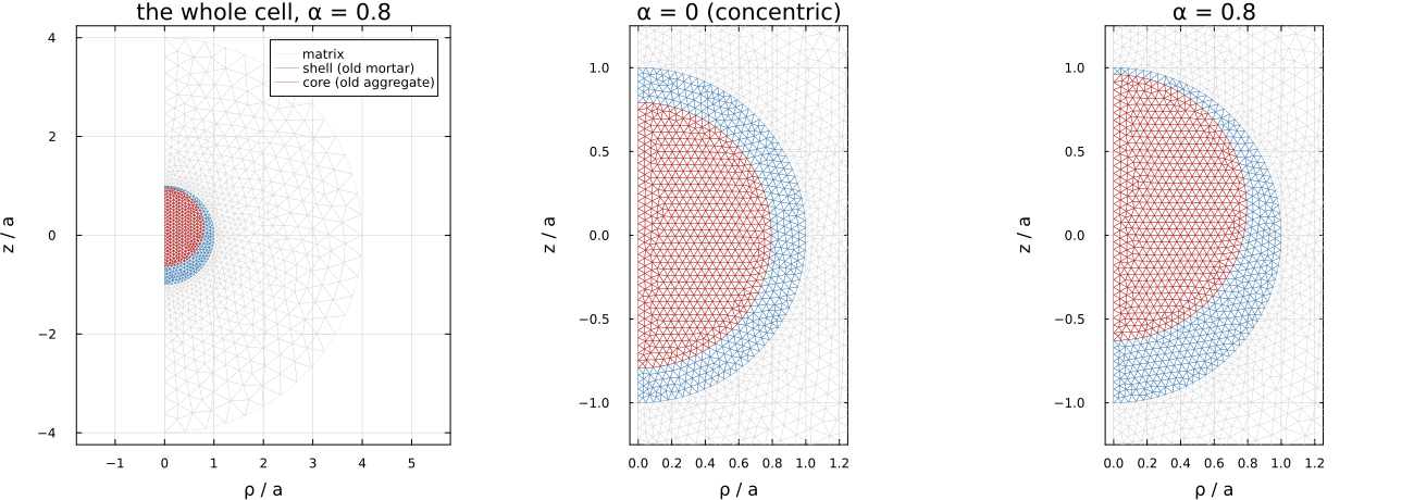
 ,  ; nradial = 14 on the left panel and nradial = 22 on the two zooms, P2 triangles.

The half-plane  , meshed with straight triangles: the core in red, the adhered mortar in blue, the surrounding matrix in gray. A node of this mesh stands for a whole circle of the three-dimensional body, and the axis on the left is a boundary of the computation, not of the body.

Left, the whole cell at   — most of it is matrix, coarsening outwards. Middle and right, the same zoom on the inclusion at   and  : with   the core already fills 79 % of the radius, so at   the shell pinches to 4 % of at the top pole and thickens to 37 % at the bottom. That contrast is the whole physical content of the eccentricity.

Element size is on the inclusion, growing to times that at the outer boundary. Because the mesh is two-dimensional, refining is cheap — nradial = 40 still solves in a fraction of a second.

Quantity	Measured	Exact	Δ
core volume	2.0930	2.0944	−0.07 %
shell volume	2.0940	2.0944	−0.02 %
cell volume	267.8380	268.0826	−0.09 %

 , nradial = 24, radius_ratio = 4: 5605 triangles, 2883 nodes (1389 in the core, 826 in the shell, 3390 in the matrix). The revolution volumes are recovered from the meridian quadrature to better than a tenth of a percent, which is the discretization of the circular arcs by straight edges.

Validation

The concentric limit

At   the morphology is the two-layer sphere and LayeredSphere gives the exact Hervé-Zaoui localization tensors. That single comparison exercises everything at once: the three Fourier modes, the axis conditions, the azimuthal projections, the    measure, the dipole correction and the Kelvin reassembly all have to be right simultaneously for it to pass — and the result must come out isotropic, although it is assembled from three separate discrete problems.

w = 0.5,  ,  ,   GPa, all Poisson ratios 0.2, nradial = 24, radius_ratio = 4.

Tensor	Part	Finite elements	Hervé-Zaoui	Δ
		0.521296	0.521262	+0.006 %
		1.532273	1.531247	+0.067 %
		4.845661	4.846822	−0.024 %
		7.815422	7.812558	+0.037 %

The assembled tensor is isotropic to   relative — although its part, its transverse shear and its in-plane shear come from three different discrete problems (modes 0, 1 and 2). Nothing forces them to agree except the correctness of the whole construction.

The correction is what makes small

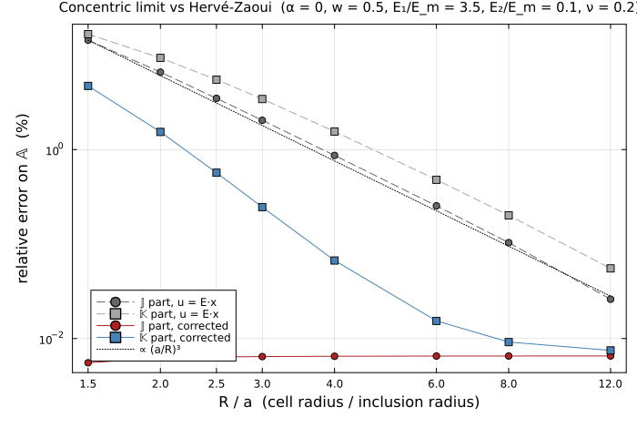
 ,  ,  ,  ,   GPa, all Poisson ratios 0.2, nradial = 24. Reference: the exact Hervé-Zaoui composite sphere.

The uncorrected cell follows the predicted line. The corrected one is flat: its residual is discretization error, not truncation, and it is already reached at  . The practical consequence is the one the paper reports — convergence at   instead of ten or more, which on a three-dimensional mesh is the difference between and   degrees of freedom.

Relative error on (%) against Hervé-Zaoui, same parameters as the figure ( , a badly degraded adhered mortar).

	,	, corrected	,	, corrected
1.5	14.383	0.006	16.675	4.720
2.0	6.599	0.006	9.328	1.538
2.5	3.484	0.006	5.494	0.569
3.0	2.042	0.006	3.429	0.246
4.0	0.867	0.006	1.553	0.067
6.0	0.254	0.007	0.479	0.015
8.0	0.103	0.007	0.201	0.009
12.0	0.026	0.007	0.055	0.007

Two different behaviors, worth separating.

The (bulk) column is the ideal case: the correction is exact to the discretization floor at every , including   where the truncated cell is off by 14 %. Under a purely spherical loading the polarization of a spherical inclusion really is a pure dipole, so the first-order correction has nothing left to miss.

The (shear) column is the realistic one: the correction removes 72 % of the bias at  , 84 % at , 93 % at , 96 % at . What is left decays much faster than the bias itself — the residual falls by 3 to 7 per step of against 1.8 to 2.4 for the uncorrected error — which is the quadrupole and beyond, the terms a first-order correction does not carry. From   on, both are at the mesh floor.

When the bias happens to be small

Reading a corrected value as always better than an uncorrected one is a mistake. For a mild contrast the deviatoric truncation bias can be a few parts in ten thousand — smaller than the correction's own higher-order residual — and the corrected shear will then look slightly worse below  . The bulk part is unaffected, and both are converged at the shipped radius_ratio = 4.

What the eccentricity does

Effective stiffness of a recycled-aggregate mortar

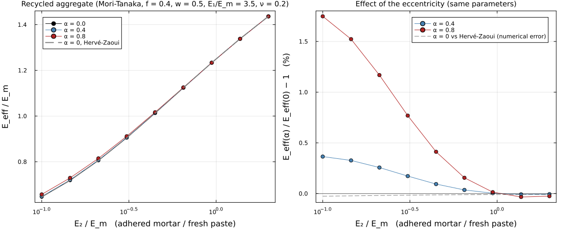
Mori-Tanaka, aggregate volume fraction  ,  ,  , all Poisson ratios 0.2,  , nradial = 20. The abscissa sweeps the quality of the adhered mortar over a decade and a half.

The engineering question of the paper: a recycled aggregate is an old natural aggregate wrapped in a shell of old mortar of uncertain, generally poor, quality. Holding the old-aggregate fraction fixed and softening the adhered mortar, how much does the concrete lose — and does it matter that the old aggregate is not centered?

Left, the effective Young modulus itself: the three eccentricities all but superpose, and the concentric one sits on the exact Hervé-Zaoui composite sphere — that superposition is the validation. Right, the same data read against the concentric case, which is the only way to see the effect at all. The gray dashed line is the numerical error of the concentric finite-element curve against the exact one, an order of magnitude below the signal.

, Mori-Tanaka, aggregate volume fraction 0.4,  ,  , all Poisson ratios 0.2.

				exact
0.100	0.6457	0.6481	0.6570	0.6459
0.211	0.8052	0.8073	0.8146	0.8054
0.447	1.0124	1.0133	1.0166	1.0125
0.944	1.2334	1.2334	1.2335	1.2335
1.372	1.3382	1.3381	1.3377	1.3383
1.995	1.4363	1.4362	1.4359	1.4364

The concentric column tracks the exact one to 0.03 % over the whole range, which is the validation. Physically: while the shell is the weak phase, moving the core off center stiffens the composite — the eccentric pattern short-circuits part of the soft mortar, so the inclusion takes up less strain. The effect is worth 1.7 % on at  , vanishes when the shell matches the paste, and changes sign beyond. What the eccentricity does not do here is make the composite noticeably anisotropic: the induced   stays below .

Equivalent conductivity of the composite particle

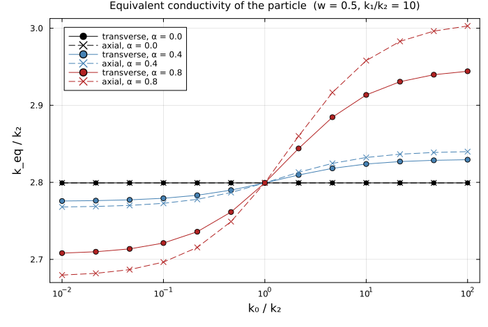
 ,   (core over shell),  , nradial = 24; the abscissa sweeps the reference medium over four decades.

The transport counterpart, reading the equivalent conductivity of the particle off  . The flat black line is the concentric particle, whose equivalent conductivity does not depend on the medium it is measured in; the eccentricity destroys that property and splits the single value into a transverse and an axial one.

read off   over the inclusion,  ,  .

		tr.	ax.	tr.	ax.
0.01	2.7993	2.7758	2.7681	2.7082	2.6797
0.1	2.7993	2.7793	2.7728	2.7212	2.6965
1	2.7993	2.7993	2.7993	2.7994	2.7994
10	2.7993	2.8238	2.8323	2.9135	2.9580
100	2.7993	2.8294	2.8398	2.9442	3.0029

The concentric column is constant: the equivalent conductivity of a concentric composite sphere is a property of the particle alone, independent of the medium it is measured in. That is a strong check — it is a theorem, not a fitted trend, and the finite-element machinery reproduces it to five digits across four decades of . The eccentric particle has no such property: its depends on , and splits into a transverse and an axial value that straddle the concentric one. All curves cross at  , where the shell and the matrix are the same material and only the core is left to see.

Using it

using MeanFieldHomogenization
import Ferrite, FerriteGmsh, Gmsh        # or: import Gridap, GridapGmsh

C_agg   = iso_stiffness(70.0 / (3 * (1 - 2 * 0.2)), 70.0 / (2 * (1 + 0.2)))
C_mortar = iso_stiffness(8.0 / (3 * (1 - 2 * 0.2)), 8.0 / (2 * (1 + 0.2)))
C₀      = iso_stiffness(20.0 / (3 * (1 - 2 * 0.2)), 20.0 / (2 * (1 + 0.2)))

incl = FEExcenteredSphere(1.0, (C_agg, C_mortar);
                          core_fraction = 0.5, eccentricity = 0.4)

A, B = fe_axi_localization(incl, C₀)     # both tensors, one solve

rve = RVE()
add_phase!(rve, :paste, Ellipsoid(1.0), Dict(:C => C₀); fraction = :rest)
add_phase!(rve, :rca, incl, Dict(:C => C₀); fraction = 0.4)
homogenize(rve, MoriTanaka(), :C)

The constituents live in the geometry object, core first then shell, as for LayeredSphere; the Dict handed to add_phase! is a placeholder the kernel ignores. Build one object per physics — a pair of Tens{4,3} for elasticity, a pair of Tens{2,3} for transport.

Discretization

FEExcenteredSphere(a, props; core_fraction, eccentricity = 0.0,
                   radius_ratio = 4.0, nradial = 24, coarsening = 6.0, order = 2)

See FEAxiMeshOptions for what each knob does.

Choosing a backend

Two finite-element libraries can perform this solve, and the physics is shared between them: the Fourier operators, the boundary data, the fixed point of the corrected boundary condition and the memoization all live in MeanFieldHomogenization.FiniteElements. What a backend supplies is a mesh, scalar Lagrange spaces, an assembly and a quadrature — nine methods in all.

import Ferrite, FerriteGmsh, Gmsh        # FerriteBackend
import Gridap, GridapGmsh                # GridapBackend

incl = FEExcenteredSphere(a, props; core_fraction, backend = GridapBackend())

Left unspecified, backend is AutoBackend, resolved at the first solve — so an inclusion can be built, stored in an RVE and passed around in a session where no finite-element package is loaded, and the informative error arrives only when a scheme actually asks for a tensor. With both stacks loaded, AutoBackend picks Ferrite. The choice is a property of the object and is pinned once solved: comparing the two means building two inclusions.

	FerriteBackend	GridapBackend
Loads	Ferrite, FerriteGmsh, Gmsh	Gridap, GridapGmsh
States the problem as	an element assembly loop	a weak form
Discretization	explicit element loop	weak form, ∫( Eᵐ(v) ⋅ D ⋅ Eᵐ(u) ρ )dΩ
Speed	≈ 5× faster	slower

Both build the same mesh, the same P2 space and the same quadrature, so they do not merely converge to the same limit — they agree to round-off, around on every tensor in both physics. That is what test/FiniteElements/test_axi_gridap.jl asserts, which makes it a sharp guard on the backend contract rather than a loose convergence check.

Which to reach for: Ferrite to run, Gridap to read or to modify. The weak form above is the equation of the axisymmetric problem transcribed, so adapting the solver to another morphology is a one-line change there and a new mesh.

Diagnostics

• fe_axi_mesh_report — cell counts and the measured revolution volumes against their exact values;

• fe_axi_breakdown — the corrected and uncorrected tensors side by side, plus the per-mode blocks;

• fe_assembly_count / fe_reset! — memoization control, shared with the finite-element crack.

Where it plugs in

The inclusion is heterogeneous (is_homogeneous_inclusion is false), so it enters through gate B of the inclusion contract with both localization tensors — the strain-side and the stress-side . They come out of the same solve, so asking for one and then the other costs one solve, not two.

Everything that consumes those two follows: Dilute, DiluteDual, MoriTanaka, Maxwell, PonteCastanedaWillis, SelfConsistent, DifferentialScheme.

Voigt and Reuss work as well — which is not automatic for a heterogeneous inclusion. A bound needs the volume average of the constituent properties over the inclusion, and the RVE cannot supply it: the phase property is a placeholder. Here the geometry fixes it exactly, w for the core and   for the shell whatever the eccentricity, so the type implements Schemes._layer_voigt / Schemes._layer_reuss and the bounds come for free.

AsymmetricSelfConsistent works whether or not the bounds do. Its iteration needs exactly what SelfConsistent needs — the same two localization tensors — and only its branch-selection heuristic, which decides once between the stiffness and the compliance form, ever consulted a bound. When no bound is available it uses the dilute estimate instead, which answers the same question ("is the composite stiffer than the matrix?") from the tensors the scheme already requires. Nothing in the asymmetric algorithm depends on Schemes._layer_voigt.

Cost and memoization

nradial = 24, radius_ratio = 4, P2, 5605 triangles: 2.05 s for a first evaluation — three assemblies, three factorizations and eight solves — and 2.5·10⁻⁵ s for a cached one. The three-dimensional cell the same problem would need is two orders of magnitude larger.

Iterative schemes ask for the tensors again at every iteration with a slightly different reference medium; FECache memoizes on the components of that medium, rounded to twelve significant digits so that arithmetic noise between two otherwise identical iterations does not miss the cache. One-shot schemes only ever hit one key.

Iterative schemes and the isotropy guard

SelfConsistent, AsymmetricSelfConsistent and DifferentialScheme re-evaluate the inclusion in their own current estimate, and the corrected boundary condition needs an isotropic reference — the anisotropic Green-function gradient (Pan-Chou, Barnett-Willis) is not implemented.

At   that is no obstacle: the estimate is isotropic, and the guard tolerates 0.01 % of deviation, deliberately loose because the finite-element tensors are themselves isotropic only to a few parts in a million — a tighter guard would refuse a perfectly legitimate problem. A family of aligned eccentric spheres, on the other hand, homogenizes to a genuinely transversely isotropic medium, and there the guard fires. Add symmetrize = IsoSymmetrize() to the phase: the scheme then hands the kernel an isotropic reference at every iteration, which also collapses a whole orientation family onto one cached solve.

Limitations

• Isotropic reference medium only, for the reason just given. Refused with a message pointing at IsoSymmetrize, and tested on the tensor's content, not on its TensND type.

• Constituents transversely isotropic about the symmetry axis (isotropy included). Any other anisotropy couples the Fourier modes, which is exactly what the formulation assumes away; it is refused rather than silently wrong.

• No automatic differentiation through the solve: the sparse factorization is Float64-only. Use finite differences for sensitivities in a geometric parameter.

• First order in . The correction keeps the leading dipole term only; the quadrupole and beyond survive in the shear part below   (see the table above). radius_ratio = 4.0 is what ships.

• One core. Several inclusions in the cell, or a non-spherical envelope, would need a different mesh — the solver itself does not care.

Reproducing this page

julia scripts/fe/make_axi_figures.jl          # figures + the tables above
julia scripts/83_fe_excentered_sphere.jl      # the runnable demonstration

and the test file that guards all of it:

julia --project=. -e 'using MeanFieldHomogenization, Ferrite, FerriteGmsh, Gmsh, Test;
                      include("test/FiniteElements/test_axi_excentered_sphere.jl")'

and, if Gridap and GridapGmsh are installed in the test environment, the cross-backend file:

julia --project=. -e 'using MeanFieldHomogenization, Ferrite, FerriteGmsh, Gmsh,
                            Gridap, GridapGmsh, Test;
                      include("test/FiniteElements/test_axi_gridap.jl")'

See also

• Finite-element inclusions — the elliptical crack, the same correction in its 3 + 3 crack form

• Custom inclusions — the contract this type satisfies

• Adding a new inclusion — the developer reference