
Symbolic spheres: closed forms with SymPy and Symbolics.jl
TensND is generic in its element type: the same tensor algebra (⊡, inv, projectors, …) runs on Float64, on SymPy.jl Sym and on Symbolics.jl Num. The classical homogenization formulas therefore come out in closed form, with numbers substituted only at the end.
Running example: a single sphere in an isotropic matrix, in three regimes — general inclusion, porous limit (scripts/29_symbolic_schemes.jl.
Setup
using MeanFieldHomogenization
using TensND
using SymPy
using Plots
gr()  # headless backend; GKSwstype is set to "100" in make.jl

@syms k0::positive μ0::positive ki::positive μi::positive f::positive ν0::real

C0 = iso_stiffness(k0, μ0)     # matrix stiffness   = TensISO{3}(3k₀, 2μ₀)
Ci = iso_stiffness(ki, μi)     # inclusion stiffness = TensISO{3}(3kᵢ, 2μᵢ)

# The Hill tensor of a sphere does not depend on its radius, so a plain
# Float64 unit sphere already gives a fully symbolic P once C0 is symbolic.
sphere = Ellipsoid(1.0)
@syms x::positive both creates the SymPy symbol x and tells the solver it is a positive real — this alone rules out a lot of spurious branches later when solve and simplify have to pick between them.
The Hill tensor and the Eshelby tensor, in closed form
hill_tensor and the double contraction ⊡ work unchanged on symbolic stiffnesses:
P = hill_tensor(sphere, C0)
S = P ⊡ C0

αP, βP = get_data(P)
αS, βS = get_data(S)
simplify(αP), simplify(βP)
(1/(3*k0 + 4*μ0), 3*(k0 + 2*μ0)/(5*μ0*(3*k0 + 4*μ0)))Every isotropic 4th-order tensor decomposes as TensND.get_data returns exactly that pair (α, β) — no further rescaling. For the sphere:
Substituting the isotropic identity
k0_of_ν0 = 2 * μ0 * (1 + ν0) / (3 * (1 - 2 * ν0))
SJ = simplify(subs(αS, k0 => k0_of_ν0))
SK = simplify(subs(βS, k0 => k0_of_ν0))
SJ, SK
((ν0 + 1)/(3*(1 - ν0)), 2*(4 - 5*ν0)/(15*(1 - ν0)))Dilute estimate — writing the master formula out by hand
The dilute strain concentration tensor and effective stiffness,
translate directly into TensND tensor algebra — inv on a TensISO is just the reciprocal of its two (α, β) scalars, so the whole computation stays in closed form:
𝕀4 = tens_Id4(Val(3), Val(Sym))
Adil = inv(𝕀4 + P ⊡ (Ci - C0))
Cdil = C0 + f * ((Ci - C0) ⊡ Adil)

k_dil, μ_dil = k_mu(Cdil)
k_dil = simplify(k_dil)
μ_dil = simplify(μ_dil)
k_dil
To confirm this by-hand derivation against the package's own scheme API, the ordinary RVE() is enough — a symbolic fraction is stored as it comes, without conversion:
rve = RVE()
add_phase!(rve, :M, sphere, Dict(:C => C0); fraction = :rest)
add_phase!(rve, :I, sphere, Dict(:C => Ci); fraction = f)

kD, μD = k_mu(homogenize(rve, Dilute(), :C))
simplify(k_dil - kD), simplify(μ_dil - μD)
(0, 0)Both differences collapse to 0 — the hand-derived formula and Dilute's internal machinery agree exactly, symbolically.
Mori–Tanaka estimate
MoriTanaka runs through the same symbolic-safe path (it only adds a volume-weighted average of concentration tensors, still pure TensISO algebra):
kMT, μMT = k_mu(homogenize(rve, MoriTanaka(), :C))
kMT = simplify(kMT)
μMT = simplify(μMT)
kMT
(
Two physical limits: porous and rigid
Substituting subs call — gives the porous limit; taking limit and oo gives the rigid limit. Both keep the whole expression symbolic in k₀, μ₀, f:
k_dil_por = simplify(subs(k_dil, ki => 0, μi => 0))
kMT_por   = simplify(subs(kMT, ki => 0, μi => 0))
k_dil_por, kMT_por
(-3*f*k0^2/(4*μ0) - f*k0 + k0, 4*k0*μ0*(1 - f)/(3*f*k0 + 4*μ0))k_dil_rig = simplify(limit(limit(k_dil, ki => oo), μi => oo))
kMT_rig = simplify(limit(limit(kMT, ki => oo), μi => oo))
k_dil_rig, kMT_rig(f*k0 + 4*f*μ0/3 + k0, (-4*f*μ0/3 - k0)/(f - 1))kMT_por is exactly the Hashin–Shtrikman upper bound for a porous solid:
Self-consistent: derived by hand, solved with solve
SelfConsistent and AsymmetricSelfConsistent are intrinsically numerical in MeanFieldHomogenization — a damped Picard/Anderson fixed-point iteration with convergence tests and positive-definiteness guards, none of which can run on a Sym scalar (a comparison like r < abstol simply has no meaning for a symbolic residual). So instead of calling the API, the self-consistent condition
is written out by hand for two isotropic spherical phases. It separates into two scalar equations, coupled through the effective moduli themselves:
@syms ksc::positive μsc::positive

κstar = 4 * μsc / 3
μstar = μsc * (9 * ksc + 8 * μsc) / (6 * (ksc + 2 * μsc))

eqk = (1 - f) * (k0 - ksc) / (k0 + κstar) + f * (ki - ksc) / (ki + κstar)
eqμ = (1 - f) * (μ0 - μsc) / (μ0 + μstar) + f * (μi - μsc) / (μi + μstar)
The general two-phase system couples eqk and eqμ through μstar — a coupled polynomial with no compact closed form. Its limits do have one. The porous limit (solve:
eqk_por = subs(eqk, ki => 0)
eqμ_por = subs(eqμ, μi => 0)
sol_por = solve([eqk_por, eqμ_por], [ksc, μsc])
ksc_por, μsc_por = sol_por[1]
length(sol_por)2The load-bearing branch must vanish exactly at the percolation threshold simplify does not collapse the nested sqrt left by solve at
for (k0v, μ0v) in ((30.0, 15.0), (90.0, 30.0), (5.0, 50.0))
    kval = N(subs(ksc_por, k0 => k0v, μ0 => μ0v, f => Sym(1) // 2))
    μval = N(subs(μsc_por, k0 => k0v, μ0 => μ0v, f => Sym(1) // 2))
    println("k₀=$k0v  μ₀=$μ0v  ->  ksc(1/2)=$kval   μsc(1/2)=$μval")
end
k₀=30.0 μ₀=15.0 -> ksc(1/2)=0 μsc(1/2)=0
k₀=90.0 μ₀=30.0 -> ksc(1/2)=0 μsc(1/2)=0
k₀=5.0 μ₀=50.0 -> ksc(1/2)=0 μsc(1/2)=0Both vanish for every (k₀,μ₀) tried — the percolation threshold does not depend on the matrix's own stiffness, only on the geometry (spheres).
For a genuinely numeric cross-check, AsymmetricSelfConsistent is run on a plain Float64 RVE and compared with the symbolic solution after substituting numbers:
k0n, μ0n, fn = 30.0, 15.0, 0.2
rve_num = RVE()
add_phase!(rve_num, :M, Ellipsoid(1.0), Dict(:C => iso_stiffness(k0n, μ0n)); fraction = :rest)
add_phase!(rve_num, :V, Ellipsoid(1.0), Dict(:C => iso_stiffness(1.0e-6, 1.0e-6)); fraction = fn)
k_sc_num, μ_sc_num = k_mu(homogenize(rve_num, AsymmetricSelfConsistent(; abstol = 1.0e-12, maxiters = 200, select_best = true), :C))

k_sc_sym = N(subs(ksc_por, k0 => k0n, μ0 => μ0n, f => fn))
μ_sc_sym = N(subs(μsc_por, k0 => k0n, μ0 => μ0n, f => fn))

(k_sc_sym, k_sc_num), (μ_sc_sym, μ_sc_num)
((16.09376442220722, 16.093766162359223), (9.160103969498827, 9.160104999516168))The two agree to solver tolerance — the hand-derived closed form is what the numerical scheme converges to, it just cannot be produced symbolically by the iteration itself.
Bonus: the same computation with Symbolics.jl
TensND does not care which symbolic engine produced its scalars. The same hill_tensor/⊡ code, run on Symbolics.jl's Num type instead of SymPy's Sym, gives the same P and S:
using Symbolics
Symbolics.@variables k0s μ0s

C0s = iso_stiffness(k0s, μ0s)
Ps = hill_tensor(sphere, C0s)
Ss = Ps ⊡ C0s

αPs, βPs = get_data(Ps)
Symbolics.simplify(αPs)
Same formula, different backend — the tensor algebra is agnostic to how the scalars got their symbolic meaning.
From formulas back to numbers
To close the loop, substitute a concrete matrix (
k_dil_por_num = subs(k_dil_por, k0 => 90.0, μ0 => 30.0)
kMT_por_num   = subs(kMT_por, k0 => 90.0, μ0 => 30.0)
ksc_por_num   = subs(ksc_por, k0 => 90.0, μ0 => 30.0)

fs = range(0.0, 0.48; length = 25)
k_dil_curve = [N(subs(k_dil_por_num, f => fv)) for fv in fs]
kMT_curve   = [N(subs(kMT_por_num, f => fv)) for fv in fs]
ksc_curve   = [N(subs(ksc_por_num, f => fv)) for fv in fs]

plt = plot(;
    xlabel = "porosity f", ylabel = "k_eff",
    legend = :topright, framestyle = :box, size = (760, 480),
    title = "Porous sphere — closed forms evaluated numerically",
    titlefontsize = 10,
)
plot!(plt, fs, k_dil_curve; label = "Dilute (closed form)", color = :blue, lw = 2)
plot!(plt, fs, kMT_curve; label = "Mori–Tanaka (closed form)", color = :green, lw = 2)
plot!(plt, fs, ksc_curve; label = "Self-consistent (closed form)", color = :purple, lw = 2)
plt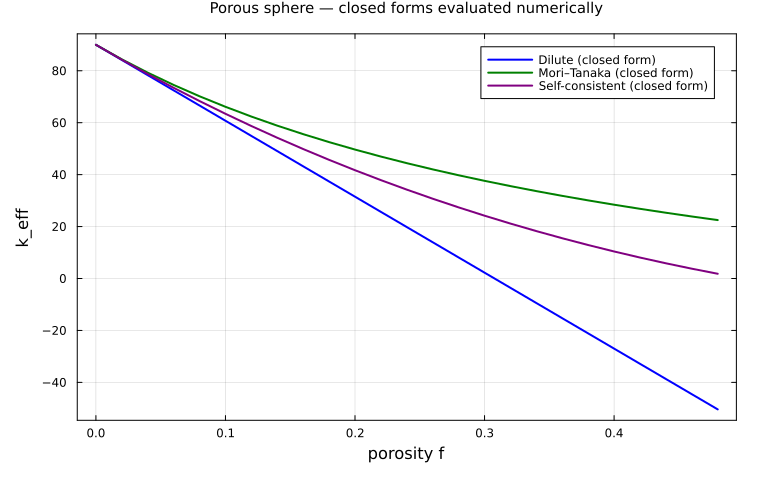
The self-consistent curve heads to zero as f → 1/2, as the percolation check predicted; dilute and Mori–Tanaka never "see" the pores connecting and stay positive throughout — the picture of the porous-materials tutorial, obtained from formulas rather than a sweep.