A lamellar porous material: swelling clays and C-S-H

Smectite clays and the calcium silicate hydrates that hold a cement paste together share a morphology: the solid is not a continuum but a stack of parallel platelets, a few nanometers apart, with water and ions in between. Two things follow, and neither is a detail.

The platelets slide freely on the interfoliar fluid — nothing transmits a tangential traction from one to the next. And they repel each other: the platelet faces carry negative charges, the counter-ions in the interfoliar water screen them imperfectly, and the resulting electrical field pushes the platelets apart with an overpressure that grows as they come closer. The macroscopic stiffness of such a material therefore has almost nothing to do with the stiffness of the solid, and almost everything to do with an electrical interaction. That is the model of [87], and this chapter derives it.

It is also the most complete example in this documentation of what the package does symbolically: not a single number is entered. Every modulus, every volume fraction is a SymPy symbol, the two scales are chained on symbols, two degenerate limits are taken with tlimit, and the closed forms come out of solve.

This chapter derives; the script also checks

scripts/46_lamellar_porous_swelling.jl runs the same derivation and then compares every intermediate result with the corresponding published equation, each comparison a simplify that must return exactly zero, plus a numerical cross-check against SelfConsistent. Here we only derive, so the page stays readable.

Running it yourself

Every code block below is executed when this documentation is built, in one session and in the order shown, so pasting them one after another into a REPL reproduces the page exactly. You need MeanFieldHomogenization, TensND, SymPy, Printf and Plots; SymPy in turn needs a working Python sympy, which the repository's docs/Project.toml already provides.

The microstructure, and the two scales

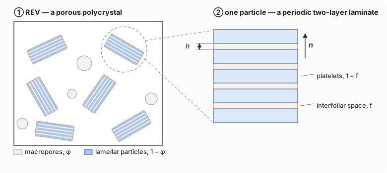
Two porosities, nested:

	Scale	What it contains	Homogenization
②	one particle	solid platelets ( ) + interfoliar space (), all normal to	exact — it is a laminate
①	the REV	particles of every orientation ( ) + macropores ()	self-consistent — no phase is a matrix

The separation of scales is what makes this legitimate: the macropores are of the order of the particles themselves, far larger than the interfoliar distance.

The interfoliar layer

Everything the model needs about the electrochemistry is packed into one scalar function. Let be the pressure in the macropores and the distance between two platelets. The interfoliar fluid, in equilibrium with the macropores, acts on the platelet faces as if its pressure were  , where the swelling overpressure depends on and on the ion concentration in the macropores. The interfoliar stress is therefore purely normal-plus-hydrostatic,

and there is no tangential term at all: that is the free sliding.

Linearizing around the reference distance is the only approximation of this step. With       the only strain measure the layer feels,

using MeanFieldHomogenization
using TensND
using SymPy
using Printf

# h₀ = reference interfoliar distance      dπ = ∂π^g/∂h at h₀
# π₀ = π^g_o, the swelling overpressure in the reference configuration
# f  = interfoliar volume fraction          p = pressure in the macropores
@syms h₀::positive dπ::real p::real π₀::real f::positive
@syms μs::positive ks::positive Π::positive    # platelet shear and bulk moduli, Π
@syms ε::real                                  # ε = n⊗n : ε_f = (h − h₀)/h₀

πg = π₀ + h₀ * dπ * ε                          # first-order expansion of π^g
σ_nn = -p - πg                                 # the n⊗n component of σ_f

    

An affine function of the strain is a linear elastic law with an initial stress, and reading the two parts off costs one derivative and one substitution:

@printf "prestress   σᵖ_nn = %s\n" string(tsubs(σ_nn, ε => 0))
@printf "stiffness  C_nnnn = %s\n" string(tdiff(σ_nn, ε))

prestress   σᵖ_nn = -p - π₀
stiffness  C_nnnn = -dπ*h₀

So the interfoliar layer behaves as a material with a single non-zero stiffness component,

positive because the swelling pressure decreases as the platelets move apart, and a prestress       . No shear stiffness, no in-plane stiffness: a spring, and nothing else.

Scale ②: the particle is a laminate

Laminate is the one cell in the package solved exactly — no reference medium, no Eshelby problem — so the particle needs no approximation beyond the one already made.

Written as it stands, though, is singular: its out-of-plane block cannot be inverted, and the laminate kernel needs that inverse. The fix is the honest one — regularize with an isotropic , then send it to zero. The platelets being incompressible adds a second limit,  . Both are genuine limit passages, taken with tlimit, which acts on the few canonical coefficients of a structured tensor and gives back the same type.

@syms κw::positive μw::positive                # the regularization, sent to 0

n̂ = (0, 0, 1)
𝟏 = TensISO{3}(one(Π))                         # second-order identity
nn = TensTI{2}(zero(Π), one(Π), n̂)             # n⊗n
W₁ = TensTI{4}(one(Π), zero(Π), zero(Π), zero(Π), zero(Π), n̂)   # n⊗n⊗n⊗n

C_platelet    = TensISO{3}(3ks, 2μs)
C_interfoliar = TensISO{3}(3κw, 2μw) + f * Π * W₁

particle = Laminate(; normal = n̂)
add_layer!(particle, :PLATELET,    Dict(:C => C_platelet);    fraction = 1 - f)
add_layer!(particle, :INTERFOLIAR, Dict(:C => C_interfoliar); fraction = f)

Laminate{Float64 → SymPyCore.Sym{PyCall.PyObject}} with 2 layer(s)
  normal : (0.0, 0.0, 1.0)
  period : 1
  layer  : :PLATELET   h = 1 - f
  layer  : :INTERFOLIAR   h = f

    is exactly the first Walpole tensor, which is why one coefficient describes completely.

Solving the cell and localizing into the interfoliar layer, then taking the two limits:

phys(t) = tsimplify(tlimit(tlimit(tlimit(t, μw, 0), κw, 0), ks, oo))

Cpar = phys(homogenize(particle, Laminated(), :C))
A_f = phys(strain_strain_loc(particle, :INTERFOLIAR))

println(typeof(Cpar), "   ← exactly TI about n, and major-symmetric (N = 5)")
println(typeof(A_f), "   ← TI too, but a concentration tensor has no major symmetry (N = 6)")

TensND.TensTI{4, SymPyCore.Sym{PyCall.PyObject}, 5}   ← exactly TI about n, and major-symmetric (N = 5)
TensND.TensTI{4, SymPyCore.Sym{PyCall.PyObject}, 6}   ← TI too, but a concentration tensor has no major symmetry (N = 6)

Both come back as exact transversely isotropic tensors about the platelet normal — six Walpole coefficients rather than 81 components, which is what keeps the rest of the page symbolically tractable. Here is the whole particle stiffness, in Kelvin-Mandel form:

KM(Cpar)

Everything the model says about a particle is in that matrix.  : the normal stiffness of the particle is the interfoliar spring, and it does not depend on . The rows and columns 4 and 5 are identically zero: no shear stiffness on any plane containing — the free sliding survives homogenization untouched. What is left is the in-plane block, carried by the platelets (the terms), plus the rank-one contribution of the spring. Those are exactly the same components read off the tensor one at a time:

@printf "ℂᵖᵃʳ_nnnn = %s\n" string(tsimplify(Cpar[3, 3, 3, 3]))
@printf "ℂᵖᵃʳ_ntnt = %s\n" string(tsimplify(Cpar[2, 3, 2, 3]))

ℂᵖᵃʳ_nnnn = Π
ℂᵖᵃʳ_ntnt = 0

The interfoliar localization tensor is just as compact — its six Walpole coefficients, in the order :

get_data(A_f)

(1/f, 1, sqrt(2)*(1 - f)/f, 0, 1, 1/f)

The tensor , and Levin

The prestress does not average trivially, and what it averages to is the tensor that carries the deviation from Terzaghi's effective stress all the way up. It is built from the interfoliar localization tensor:

Bπ = tsimplify(f * (nn ⊡ A_f))
get_data(Bπ)          # (transverse, axial) coefficients of  a nT + b n⊗n

(1 - f, 1)

that is        — the axial coefficient is 1 and the transverse one is  . Levin's theorem then gives the particle's state equation; only the interfoliar layer is prestressed, so a single term survives:

σp = -p * 𝟏 - π₀ * nn                    # only the interfoliar layer is prestressed
Σ_pre = tsimplify(f * (σp ⊡ A_f))
a, b = get_data(Σ_pre)                   # transverse and axial coefficients
@printf "f σᵖ : 𝔸_f = (%s) (𝟏 − n⊗n) + (%s) n⊗n\n" string(sympy.collect(a, π₀)) string(sympy.collect(b, π₀))

f σᵖ : 𝔸_f = (-p + π₀*(f - 1)) (𝟏 − n⊗n) + (-p - π₀) n⊗n

Transverse   , axial  : that is exactly    , and the particle's state equation reads

Scale ①: the porous polycrystal

The REV has no matrix — particles of every orientation and macropores of zero stiffness, all of them spherical in shape — so the self-consistent scheme is the natural closure, with the Hill tensor of a sphere in the running isotropic estimate   .

The orientation average is the part usually done by quadrature. It does not have to be: the average of a tensor over SO(3) is a closed-form linear map on its Walpole coefficients, and that is precisely what isotropify computes — the very routine the package runs behind symmetrize = :iso. Nothing is discretized here.

@syms κ::positive μ::positive φ::positive

C_ac = TensISO{3}(3κ, 2μ)
sphere = Ellipsoid(1.0)
A_par = strain_strain_loc(sphere, Cpar, C_ac)    # (𝕀 + ℙ:(ℂᵖᵃʳ − ℂᵃᶜ))⁻¹

# The macropores have zero stiffness: they contribute nothing to ⟨ℂ:𝔸⟩, so the
# self-consistent condition ℂᵃᶜ = ⟨ℂ:𝔸⟩ reads
CA = isotropify(Cpar ⊡ A_par)          # the exact SO(3) average — a TensISO
residual = get_data(C_ac - (1 - φ) * CA)   # two scalars: the 𝕁 and 𝕂 parts
println(typeof(CA), " ⇒ ", length(residual), " scalar equations in (κ, μ)")

TensND.TensISO{4, 3, SymPyCore.Sym{PyCall.PyObject}, 2} ⇒ 2 scalar equations in (κ, μ)

The same average, applied to  , gives the macroscopic Terzaghi deviation , which is isotropic and hence a single number:

g_expr = (1 - φ) * get_data(isotropify(Bπ ⊡ A_par))[1]
typeof(g_expr)        # one scalar, still a function of κ, μ, φ, f, μs and Π

SymPyCore.Sym{PyCall.PyObject}

The leading order in

Osmotic swelling puts orders of magnitude below the elasticity of the solid, so the interesting regime is  . Rather than send a modulus to infinity inside a large rational fraction, nondimensionalize:   with  , then   and  . Both and then leave the equations of their own accord.

@syms t::positive x::positive y::positive

reduce_lead(z) = tsimplify(
    sympy.cancel(
        sympy.limit(
            sympy.cancel(sympy.together(tsubs(z, κ => Π * x, μ => Π * y, μs => Π / t))),
            t, 0, "+",
        )
    )
)

eq1 = tsimplify(sympy.cancel(reduce_lead(residual[1]) / Π))
eq2 = tsimplify(sympy.cancel(reduce_lead(residual[2]) / Π))
gA = reduce_lead(g_expr)

println("free symbols of the reduced system : ", eq1.free_symbols ∪ eq2.free_symbols)

free symbols of the reduced system : Set(SymPyCore.Sym{PyCall.PyObject}[x, y, φ])

There they are, in full — two rational equations in with as the only parameter:

eq1

eq2

Π has canceled and f is nowhere to be seen. That is the physical content of the model: at leading order the macroscopic elasticity depends on neither the platelet elasticity nor the interfoliar porosity — only on the repulsive interaction, through , and on how much room the macropores leave.

solve takes them from here. The system has several roots; the physical one is the branch with a positive shear modulus:

branches = sympy.solve([eq1, eq2], [x, y]; dict = true)
sol = first(
    b for b in branches
        if (v = Float64(tsubs(tsimplify(b[y]), φ => Sym(1) / 10)); isfinite(v) && v > 0)
)
xs, ys = tsimplify(sol[x]), tsimplify(sol[y])
sympy.factor(ys)

so that

ν_ac = tsimplify((3xs - 2ys) / (2 * (3xs + ys)))
g_ac = tsimplify(sympy.factor(tsubs(gA, x => xs, y => ys)))

@printf "μᵃᶜ / Π = %s\n" string(sympy.factor(ys))
@printf "νᵃᶜ     = %s\n" string(sympy.factor(ν_ac))
@printf "g(φ)    = %s\n" string(g_ac)
@printf "roots of μᵃᶜ : %s\n" string(sympy.solve(sympy.numer(sympy.cancel(ys)), φ))

μᵃᶜ / Π = -(φ + 2)*(4*φ - 1)/(16*φ*(φ + 1))
νᵃᶜ     = (17*φ + 2)/(5*(5*φ + 2))
g(φ)    = (φ + 2)*(4*φ - 1)/(3*φ - 2)
roots of μᵃᶜ : SymPyCore.Sym{PyCall.PyObject}[1/4]

The macroscopic state equation is then

the last term being the departure from Terzaghi's principle — a macroscopic stress that exists with no macroscopic strain and no pore pressure, produced entirely by the repulsion between platelets at the nanometer scale.

Reading the result

using Plots
gr()  # headless backend; GKSwstype is set to "100" in make.jl

φs = range(0.004, 0.2495; length = 200)
μ̂(v) = Float64(tsubs(ys, φ => Sym(v)))
ĝ(v) = Float64(tsubs(g_ac, φ => Sym(v)))

p1 = plot(φs, μ̂.(φs); lw = 2, label = "", ylims = (0, 8),
          xlabel = "macroporosity  φ", ylabel = "μᵃᶜ / Π")
vline!(p1, [0.25]; ls = :dash, lc = :gray, label = "percolation, φ = 1/4")
p2 = plot(φs, ĝ.(φs); lw = 2, label = "",
          xlabel = "macroporosity  φ", ylabel = "g")
vline!(p2, [0.25]; ls = :dash, lc = :gray, label = "percolation, φ = 1/4")
plot(p1, p2; layout = (1, 2), size = (900, 340),
     left_margin = 6Plots.mm, bottom_margin = 6Plots.mm, top_margin = 3Plots.mm)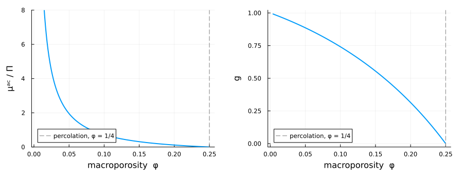

Three things are worth stating plainly.

• The macroscopic shear modulus is set by an electrical interaction. It carries a factor and nothing of . Shearing one particle parallel to its platelets costs nothing on its own — the platelets simply slide — so the only resistance comes from the normal stiffness of the neighboring particles, whose platelets are not aligned with it. The material is stiff because it is disordered.

• decreases with and vanishes at  , the percolation threshold of the self-consistent scheme, and the coefficient vanishes there too: past that porosity the particles no longer form a connected skeleton and the assembly carries no deviatoric stress at all. The value is the scheme's, not nature's, and should be read as indicative.

•   is a measurable departure from Terzaghi. An effective stress    still contains   : a swelling clay left to itself, at constant pore pressure, is under stress.