Nonlinear homogenization: the secant method on a porous plastic solid

Every scheme in MeanFieldHomogenization is linear: it maps phase stiffnesses to an effective stiffness. A nonlinear material can still be treated with those same tools, by replacing each phase with a linear comparison material whose modulus is re-estimated from the strain the phase actually sees. This page walks through one such construction — the modified secant method ([74], [75]) — on the classical test case: a porous solid whose matrix is elastic–perfectly plastic, loaded hydrostatically.

Two ingredients make it work, and both already exist in the package:

1. the composite sphere assemblage (LayeredSphere), which resolves the radial profile of the plastic strain by subdividing the solid into concentric shells, each carrying its own secant modulus;

2. automatic differentiation through a self-consistent scheme, which delivers the second moment of the strain in each shell without ever touching a local field.

The nonlinear closure, and why a derivative gives it

Write the macroscopic strain as    with    its volumetric part and its deviator. For an isotropic effective behavior of moduli the macroscopic elastic energy is

Now let be the shear modulus of shell , of volume fraction . Differentiating with respect to — at fixed macroscopic strain, so that only the explicit dependence survives — gives the second moment of the deviatoric strain in that shell ([76], [74]):

This is the whole point of the method: a quantity that looks local — the quadratic average of the strain inside one shell — is obtained from the derivative of the effective moduli, which ForwardDiff supplies exactly.

Writing for the resulting equivalent deviatoric strain,  , a von Mises solid of elastic shear modulus responds with the secant modulus

Where the square root of 2/3 comes from

is the yield stress in simple tension, which is how a von Mises criterion is normally quoted. The quantity the secant closure actually caps is the norm of the deviatoric stress  , and under simple tension     the deviator has norm   , not . Yielding therefore reads   . Dropping that factor rescales the whole plastic branch by   — enough to make a converged estimate look like a systematic 20 % overestimate.

The shells are coupled through , so this is a fixed point on the vector — solved below by direct iteration.

using MeanFieldHomogenization
using TensND
using ForwardDiff
using Printf
using Plots
gr()  # headless backend; GKSwstype is set to "100" before Literate runs

Plots.GRBackend()

§1 The porous material

The solid is elastic–perfectly plastic: bulk modulus , shear modulus , yield stress (a threshold on the deviatoric stress norm  ). The porosity is . Plasticity only enters through ; the bulk modulus never changes, since a von Mises solid is plastically incompressible.

const KS = 2.0e3      # bulk modulus of the solid phase
const MUS = 1.0e3     # shear modulus of the solid phase
const SIG0 = 1.0      # yield stress
const FPORE = 0.1     # porosity

0.1

The RVE is a composite sphere: a void core of volume fraction , surrounded by shells of equal volume fraction   . Radii follow from cumulative volume fractions,  , the outer radius being 1.

A void is a very soft solid, not an empty one

The shell recurrence inverts a transfer matrix layer by layer, which is singular for an exactly zero stiffness. The core is therefore given a small positive modulus — the same TINY convention the strength scripts use for water and air (scripts/README.md). At its effect on the results below is far under the plotting resolution.

The shells are not a discretization of the geometry — the composite sphere is exact for any number of them. They are a discretization of the plastic zone: each shell carries its own secant modulus, so a plastic front moving outwards from the cavity is resolved shell by shell. Cut open, with the void core at the center:

include(joinpath(pkgdir(MeanFieldHomogenization), "scripts", "common", "docviz.jl"))

let n = 5, f = FPORE
    radii = ntuple(i -> i == 1 ? f^(1 / 3) : (f + (1 - f) * (i - 1) / n)^(1 / 3), n + 1)
    ls = LayeredSphere(radii, ntuple(i -> iso_stiffness(KS, MUS), n + 1))
    plotly_scene(
        shape_traces(ls; colors = ["#ffffff", "#f0ad4e", "#e8a33d", "#d4913a",
            "#c0392b", "#8a2e22"]);
        uid = "secant-shells", height = 450,
        title = "Composite sphere: void core (f = $f) and $n plastic shells"
    )
end

The same geometry, parameterized by the shell moduli rather than fixed, is what the secant iteration below rebuilds at every step:

function porous_sphere(μs, f)
    n = length(μs)
    T = eltype(μs)
    tiny = T(1.0e-8) * KS
    # Radii: the core carries f, then each shell adds (1-f)/n.
    radii = ntuple(i -> i == 1 ? f^(1 / 3) : (f + (1 - f) * (i - 1) / n)^(1 / 3), n + 1)
    # Every layer must share one element type, or ForwardDiff cannot promote
    # the tuple when only the shells carry Duals.
    moduli = (
        TensISO{3}(3tiny, 2tiny),
        ntuple(i -> TensISO{3}(3 * T(KS), 2 * μs[i]), n)...,
    )
    return LayeredSphere(radii, moduli)
end

porous_sphere (generic function with 1 method)

The composite sphere fills the whole RVE (volume fraction 1) and is homogenized self-consistently: the reference medium is the effective medium itself, which is what makes the assemblage a model of the porous material rather than of dilute voids in a matrix.

The property declared for the phase is irrelevant here — for a heterogeneous inclusion MeanFieldHomogenization reads the moduli from the inclusion, not from the phase dictionary — but one must be supplied, so the solid stiffness is used.

function kmu_hom(μs, f)
    C_ref = TensISO{3}(3 * eltype(μs)(KS), 2 * μs[1])
    rve = RVE()
    add_phase!(rve, :M, Ellipsoid(1.0, 1.0, 1.0), Dict(:C => C_ref); fraction = :rest)
    add_phase!(rve, :I, porous_sphere(μs, f), Dict(:C => C_ref); fraction = 1.0)
    return collect(k_mu(homogenize(rve, SelfConsistent(), :C)))
end

kmu_hom (generic function with 1 method)

§2 The secant closure by automatic differentiation

One ForwardDiff.jacobian call gives the two rows and at once — the whole nonlinear closure, in one line.

function secant_update(μs, f, Ev, Ed2)
    n = length(μs)
    J = ForwardDiff.jacobian(m -> kmu_hom(m, f), μs)   # row 1: k, row 2: μ
    fi = (1 - f) / n
    ε₀ = sqrt(2/3) * SIG0 / (2 * MUS)
    return map(1:n) do i
        x = sqrt(max(0.0, (0.5 * J[1, i] * Ev^2 + J[2, i] * Ed2) / fi))
        x ≤ ε₀ ? MUS : sqrt(2/3) * SIG0 / (2x)
    end
end

secant_update (generic function with 1 method)

Direct iteration converges in a few tens of steps; converged is returned so that a silently unconverged point can never be plotted as if it were a result.

function solve_secant(μ0, f, Ev, Ed2; tol = 1.0e-9, maxiter = 200)
    μ = copy(μ0)
    for _ in 1:maxiter
        μnew = secant_update(μ, f, Ev, Ed2)
        Δ = maximum(abs.(μnew .- μ) ./ μ)
        μ = μnew
        Δ < tol && return μ, true
    end
    return μ, false
end

solve_secant (generic function with 1 method)

§3 The stress–strain response

Loading is purely hydrostatic:  , so   and the response is read on the mean stress  . Note that plasticity develops all the same: the void makes the local strain deviatoric even under a purely volumetric macroscopic strain, and it is that local deviator which yields.

Each strain step starts from the previous converged (continuation), which keeps the iteration count low along the whole curve.

function response(n, f, Evs)
    μ = fill(MUS, n)
    Σm = Float64[]
    allok = true
    for Ev in Evs
        μ, ok = solve_secant(μ, f, Ev, 0.0)
        allok &= ok
        push!(Σm, kmu_hom(μ, f)[1] * Ev)
    end
    return Σm, allok
end

Evs = range(0.0, 4.0e-3; length = 51)[2:end]
shells = (1, 2, 5, 20)

curves = Dict{Int, Vector{Float64}}()
for n in shells
    Σm, ok = response(n, FPORE, Evs)
    ok || @warn "n = $n: fixed point did not converge at every strain step"
    curves[n] = Σm
    @printf("n = %2d shells : Σm plateau = %.4f σ₀\n", n, Σm[end] / SIG0)
end

n =  1 shells : Σm plateau = 1.8974 σ₀
n =  2 shells : Σm plateau = 1.6837 σ₀
n =  5 shells : Σm plateau = 1.5708 σ₀
n = 20 shells : Σm plateau = 1.5378 σ₀

The curves show the two regimes: a common elastic branch of slope , then a plateau once the whole solid has yielded. Refining the radial discretization lowers the plateau and converges.

plt = plot(
    xlabel = "volumetric strain Eᵥ", ylabel = "mean stress Σₘ / σ₀",
    legend = :bottomright, title = "Porous plastic solid, hydrostatic loading (f = $FPORE)",
)
for n in shells
    plot!(plt, Evs, curves[n] ./ SIG0; marker = :circle, markersize = 2,
        label = "n = $n shell" * (n > 1 ? "s" : ""))
end
hline!(plt, [(2 / 3) * log(1 / FPORE)]; linestyle = :dash, color = :black,
    label = "hollow sphere, (2/3)ln(1/f)")
plt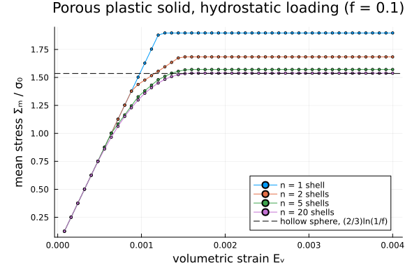

§4 What the plateau converges to

For a rigid–perfectly plastic hollow sphere under hydrostatic loading, limit analysis gives the exact collapse stress   — the hydrostatic point of the Gurson criterion ([77]). Refining the radial discretization drives the secant estimate onto it:

@printf("\nexact rigid-plastic hollow sphere : %.4f σ₀\n", (2 / 3) * log(1 / FPORE))
for n in shells
    @printf(
        "  n = %2d : %.4f σ₀   (%+.1f %%)\n", n, curves[n][end] / SIG0,
        100 * (curves[n][end] / SIG0 / ((2 / 3) * log(1 / FPORE)) - 1)
    )
end

exact rigid-plastic hollow sphere : 1.5351 σ₀
  n =  1 : 1.8974 σ₀   (+23.6 %)
  n =  2 : 1.6837 σ₀   (+9.7 %)
  n =  5 : 1.5708 σ₀   (+2.3 %)
  n = 20 : 1.5378 σ₀   (+0.2 %)

So the number of shells is not a numerical detail — it is the model, and the two ends of the sweep are both meaningful.

A single shell reproduces the classical variational estimate. With   the second moment is taken over the whole solid at once, which is exactly the linear-comparison construction of the variational / modified secant method ([75], [74]): one uniform secant modulus for the entire matrix. The resulting plateau matches   to five digits — verified here at  , and :

@printf("\n  n = 1 plateau                    : %.5f σ₀\n", curves[1][end] / SIG0)
@printf("  (2/3)·(1-f)/√f                   : %.5f σ₀\n", (2 / 3) * (1 - FPORE) / sqrt(FPORE))

  n = 1 plateau                    : 1.89737 σ₀
  (2/3)·(1-f)/√f                   : 1.89737 σ₀

That estimate sits about 24 % above the exact collapse load at this porosity: a uniform secant modulus cannot represent a solid that yields near the void long before it yields far from it, and the quadratic average of over the whole shell overstates the dissipation.

Resolving the radial profile removes that gap. Each shell then carries its own secant modulus, the plastic front is free to progress outwards from the void, and the estimate converges to the exact limit — within 0.2 % at  . Over the range computed here the approach is monotone and always from above.

Where the derivative came from

Nothing above ever evaluated a local field. The second moment of the strain in each shell came out of ForwardDiff.jacobian applied to a self-consistent homogenization — the same sensitivity machinery used in the sensitivities tutorial for parameter studies. A nonlinear constitutive law is, from the package's point of view, just one more consumer of that derivative.

---

This page was generated using Literate.jl.