Homogenization schemes

The MeanFieldHomogenization.Schemes module provides ten classical mean-field homogenization schemes plus a RVE container holding the phases with their geometries, properties and volume fractions or crack densities.

Building an RVE

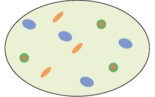
An RVE is the morphological picture, written down: phases, each with a geometry, properties and an amount. No phase is singled out. Whether one of them acts as a matrix is not a property of the microstructure but of the model applied to it, and it is stated on the scheme — see Who is the matrix? below.

using MeanFieldHomogenization, TensND

rve = RVE()
add_phase!(rve, :M, Ellipsoid(1.0),
           Dict(:C => TensISO{3}(30.0, 10.0)); fraction = :rest)
add_phase!(rve, :I, Ellipsoid(1.0, 1.0, 0.5),
           Dict(:C => TensISO{3}(60.0, 20.0)); fraction = 0.2)
add_phase!(rve, :CRACK, PennyCrack(1.0),
           Dict(:C => TensISO{3}(30.0, 10.0)); density  = 0.05)

fraction = :rest declares the phase that takes up the volume the others leave, 1 - Σ f. It is pure bookkeeping — it says nothing about morphology — and an RVE may equally well have none, with every fraction given explicitly.

Volume fractions are stored at the RVE level (not on the inclusions), so a single inclusion remains usable for localization-tensor calculations without any RVE machinery (hill_tensor, strain_strain_loc, …). Crack densities are excluded from the unit sum: a flat crack's volume vanishes in the penny limit while its density stays finite.

Who is the matrix?

Three independent things used to travel together under the name "matrix". They are now stated separately.

The phase that takes up the complement is bookkeeping, declared on the phase with fraction = :rest. Which fractions are given and which is derived is governed by the RVE's AbstractFractionClosure:

RVE()                       # inferred: ComplementFraction() if a phase says
                            # `fraction = :rest`, StrictFractions() otherwise
RVE(; closure = :strict)    # the declared fractions must already sum to 1
RVE(; closure = :rescale)   # they are relative proportions: 2, 3, 5 → 0.2, 0.3, 0.5

The reference medium — the infinite medium each inclusion is embedded in — is a modeling choice, and belongs to the scheme:

homogenize(rve, MoriTanaka(:M), :C)   # :M is the reference medium
homogenize(rve, MoriTanaka(:I), :C)   # so is :I — a different composite
homogenize(rve, MoriTanaka(), :C)     # unnamed: the `:rest` phase, if there is one

Naming nothing works only when the RVE designates a complement phase; otherwise the scheme errors and lists the candidates, because guessing would silently return a different composite. Which schemes need one:

Needs a reference medium	Does not
Dilute, DiluteDual, MoriTanaka, Maxwell, PonteCastanedaWillis, DifferentialScheme, AsymmetricSelfConsistent	Voigt, Reuss, SelfConsistent, Laminated

The homogeneous solid of microporomechanics is a third notion again, and biot_tensor / poroelastic_parameters take it as solid =.

A ParticleAssembly does keep a matrix

add_matrix! still exists, on ParticleAssembly only. There it is structural rather than a modeling choice: both N-body models are written against a reference medium the particles sit in.

Calling a scheme

C_voigt = homogenize(rve, Voigt())         # type-instance
C_mt    = homogenize(rve, :mt)             # Symbol shortcut (lowercase canonical)
C_sc    = homogenize(rve, SelfConsistent(; abstol = 1e-12, maxiters = 200))

Every scheme takes the optional kwarg property = :C (default, elasticity) or property = :K (conductivity). Iterative schemes also accept abstol, reltol, maxiters, damping, verbose and select_best — see Solver tolerances for what they mean and, in particular, for why reltol is usually the one that decides when the iteration stops.

Long form	Short / ECHOES code
:voigt	:v, :V, :Voigt, :VOIGT
:reuss	:r, :R …
:dilute	:dil, :DIL
:dilute_dual	:dild, :DILD
:mori_tanaka	:mt, :MT
:maxwell	:max, :MAX
:ponte_castaneda_willis	:pcw, :PCW
:self_consistent	:sc, :SC
:asymmetric_self_consistent	:asc, :ASC
:differential	:diff, :DIFF
:cluster	:cluster_model, :ClusterModel, :CLUSTER
:eim	:EIM, :equivalent_inclusion

The last two act on a different cell

:cluster and :eim are N-body schemes: they resolve the interaction between individual inclusions and therefore need their positions, which an RVE does not carry. They act on a ParticleAssembly instead — see the particle-assembly page.

Distribution shape (Maxwell, PCW)

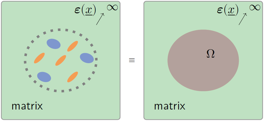
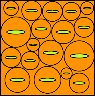
Two schemes take a second shape, describing how the inclusions are placed rather than what they look like. Maxwell reads it as the envelope of a cluster that is replaced by one equivalent inclusion; PCW reads it as a distribution ellipsoid around each inclusion, forbidding closer approach:

Maxwell	Ponte Castañeda–Willis

rve = RVE(; distribution_shape = Ellipsoid(1.0, 1.0, 0.3))   # oblate outer
add_phase!(rve, :M, Ellipsoid(1.0), Dict(:C => TensISO{3}(30.0, 10.0)); fraction = :rest)
add_phase!(rve, :I, Ellipsoid(1.0), Dict(:C => TensISO{3}(60.0, 20.0));
           fraction = 0.3)
homogenize(rve, Maxwell())

The distribution_shape field is wrapped in UniformDistribution. A future PairwiseDistribution (Willis 1982) can be added without breaking the public API — see AbstractDistributionShape.

It belongs to the RVE, and it has no default

Two questions that look alike, and answer differently.

Why is it on the RVE and not on the scheme? Because it is microstructure. The distribution ellipsoid describes the ellipsoidal symmetry of the two-point statistics of the actual medium [28] — a measurable property of the material, like a phase's shape or its volume fraction. That is what separates it from the matrix, which left the RVE in v0.8.0: naming a reference medium is a modeling decision, and the same microstructure is a matrix/inclusion composite under Mori–Tanaka and a matrix-free aggregate under the self-consistent scheme. No such thing is true here. The spatial statistics of an RVE do not change according to which scheme is about to read them.

Then why do only two schemes read it? For the same reason Voigt reads no shape at all: a cruder estimate uses less of the microstructure. Being ignored by nine schemes out of eleven is the normal condition of microstructural data, not a sign that the field is in the wrong place.

An undeclared distribution shape is an error

Where the field does differ from a phase geometry is that it has no harmless default. A spherical distribution makes Maxwell and PCW coincide exactly with Mori–Tanaka. Supplying one silently — which is what this field used to do — therefore answered the scheme whose whole purpose is a non-spherical distribution with the estimate it generalizes, and said nothing about it.

So an RVE that declares none raises, the way a matrix-based scheme raises when no phase can play the reference medium:

rve = RVE()                                    # no distribution declared
homogenize(rve, PonteCastanedaWillis())        # ArgumentError, naming the collapse

A spherical distribution remains a perfectly legitimate modeling choice. It just has to be the caller's:

rve = RVE(; distribution_shape = Ellipsoid(1.0))
homogenize(rve, PonteCastanedaWillis()) ≈ homogenize(rve, MoriTanaka())   # true, and now on purpose

This is also the quickest way to check that the option is wired correctly.

Iterative solvers

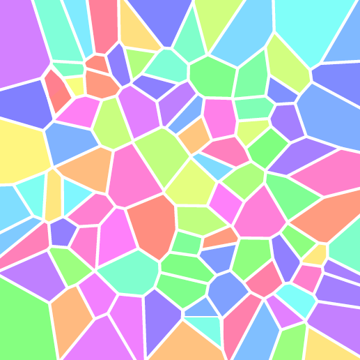
The self-consistent schemes describe the other morphology: no phase is a matrix, every phase is embedded in the medium being sought — which is why a polycrystal or a granular assembly is homogenized this way and not by Mori–Tanaka. SelfConsistent has no reference-medium field at all, and an RVE whose fractions are all declared needs no complement phase either:

poly = RVE(; closure = :strict)
add_phase!(poly, :A, Ellipsoid(1.0), Dict(:C => C_A); fraction = 0.4)
add_phase!(poly, :B, Ellipsoid(1.0), Dict(:C => C_B); fraction = 0.6)
homogenize(poly, SelfConsistent(), :C)

The fixed point has to start somewhere, and with no phase distinguished the seed is stated on the scheme: init accepts :voigt, :reuss, a phase name or an explicit tensor. Unset, it is the :rest phase when there is one and the Voigt average otherwise — the latter is what lets the RVE above be solved at all.

homogenize(rve, SelfConsistent())                            # built-in damped Picard (default)
homogenize(rve, SelfConsistent(; algorithm = NewtonDefault()))  # built-in Newton-Raphson (dependency-free)

# With NonlinearSolve.jl loaded, any SciML algorithm can be selected:
using NonlinearSolve
homogenize(rve, SelfConsistent(; algorithm = NewtonRaphson(),
                                abstol = 1e-12, maxiters = 200))
homogenize(rve, SelfConsistent(; algorithm = TrustRegion()))

# Auto-resolving: uses NonlinearSolve.TrustRegion() when the extension
# is active, falls back to the built-in NewtonDefault otherwise:
homogenize(rve, SelfConsistent(; algorithm = AutoNonlinear()))

Three solver families are available for SelfConsistent / AsymmetricSelfConsistent:

Solver	Dependency	Jacobian	Use when
AndersonDefault (default)	none	— (damped Picard)	always, and especially near a bifurcation: the positive-definite guard and select_best track the physical branch
NewtonDefault	none	ForwardDiff on the canonical components	a smooth, well-separated fixed point; fails on complex moduli
NonlinearSolve.jl algorithm, or AutoNonlinear	MeanFieldHomogenizationNonlinearSolveExt	the SciML algorithm's own	you already depend on SciML and want TrustRegion, LevenbergMarquardt, …

AutoNonlinear resolves to a SciML algorithm when the extension is loaded and to the built-in Newton otherwise. It is not the default: a root-finder is not guaranteed to track the physical branch through the SC bifurcation the way the Picard guard does.

All three are ForwardDiff-compatible — differentiating homogenize through a NonlinearSolve algorithm uses an implicit-function-theorem lift, so no nested Duals ever form (see derivative and the Nonlinear solvers tutorial).

Solver tolerances

Every iterative solver in the package stops on the additive SciML convention

with ‖·‖ the Frobenius norm of the tensor — the same quantity whatever the symmetry class and whatever the algorithm, so that one abstol expresses one requirement.

Family	abstol	reltol	maxiters
SelfConsistent, AsymmetricSelfConsistent	1e-12	1e-8	100
ALV (ageing-viscoelastic) counterparts	1e-10	1e-8	200
DifferentialScheme (forwarded to OrdinaryDiffEq)	1e-8	1e-6	→ solve
hill_tensor cubature backends	1e-8	1e-6	10^6

abstol alone will not tighten a stiffness iteration

A stiffness carries a physical magnitude — tens of GPa — so reltol · ‖C‖ is of order 1e-7 at the default reltol. Lowering abstol to 1e-15 and leaving reltol alone therefore changes nothing: the relative term still decides. Tighten both, or set abstol = 0 for a purely relative test:

SelfConsistent(; abstol = 0.0, reltol = 1e-14, maxiters = 50_000)

This matters wherever a converged value is read off rather than plotted — percolation thresholds above all, where the fixed point slows down and a loose tolerance returns a small positive stiffness that merely tracks the tolerance itself.

abstol = 0 is also the exact translation of Echoes' epsrel, whose fixed point tested ‖X - X_old‖ > epsrel · ‖X_old‖ and had no absolute term at all (see Coming from Echoes).

select_best returns the best iterate seen rather than the last one — worth having when Picard oscillates around a high-contrast fixed point. Non-convergence is reported through @debug, not @warn: set JULIA_DEBUG=MeanFieldHomogenization or pass verbose = true to surface it.

Differential scheme

The differential scheme applies the dilute step over and over, updating the reference medium each time — the loop is drawn in The differential scheme. Two knobs follow from that loop: how many steps (nsteps), and in which order the phases are grown (the trajectory).

Trajectories

homogenize(rve, DifferentialScheme())                             # Proportional (default)
homogenize(rve, DifferentialScheme(; trajectory = Sequential(:I1, :I2)))
homogenize(rve, DifferentialScheme(; trajectory = Path(:I1 => τ -> τ^2, :I2 => τ -> 2τ - τ^2)))
homogenize(rve, DifferentialScheme(; trajectory = CustomPath(:I => collect(range(0.0, 1.0; length = 101)))))

Every trajectory takes either a Dict or the pair form shown above. For multi-phase RVEs the trajectory choice is physical — the schemes agree in the dilute limit and diverge at finite fractions. Cracks follow the trajectory like any other phase, their target being the final density; because they carry no volume they enter the volume balance differently (see The differential scheme).

Stiffness or compliance

homogenize(rve, DifferentialScheme(), :C)                             # stiffness (default)
homogenize(rve, DifferentialScheme(; formulation = :compliance), :C)  # compliance

Both integrate the same trajectory and return the same declared property; they differ only in which variable carries the solver's error control. Prefer :compliance for a medium softening towards percolation (porous, cracked), :stiffness for a stiffening one.

Solver control

The ODE is solved by OrdinaryDiffEq. nsteps sets only the density of saved points along τ; the step size is adaptive and governed by the tolerances.

DifferentialScheme(; alg = Vern9(), abstol = 1e-12, reltol = 1e-10)
DifferentialScheme(; maxiters = 10^7)   # unrecognised kwargs go to `solve`

Implicit algorithms need a non-AD Jacobian (Rosenbrock23(autodiff = AutoFiniteDiff())): the RHS calls the Hill-tensor backends, which are not differentiable with respect to the ODE state.

To follow the effective property along the incorporation path rather than at τ = 1 only:

τ, Cs = differential_path(rve, DifferentialScheme(; nsteps = 200), :C)
ks = [k_mu(C)[1] for C in Cs]

Frequency-domain viscoelasticity

δ = 0.05
rve = RVE()
add_phase!(rve, :M, Ellipsoid(1.0), Dict(:C => TensISO{3}(30.0 + δ * im, 10.0 + 0.5δ * im)); fraction = :rest)
add_phase!(rve, :I, Ellipsoid(1.0),
           Dict(:C => TensISO{3}(60.0 + δ * im, 20.0 + 0.5δ * im));
           fraction = 0.3)

C_eff = homogenize(rve, MoriTanaka())   # eltype(C_eff) == ComplexF64

All schemes propagate Complex{Float64} through their tensor algebra. The Im → 0 limit consistently recovers the real-modulus result.

Time-domain ageing viscoelasticity

For full time-domain ALV homogenization (relaxation / creep kernels R(t,t') / J(t,t'), possibly ageing), pass a ViscoLaw property and a times grid to homogenize_alv:

function R_iso(t, tp)
    α = 3 * (3.0 + 2.0 * exp(-(t - tp) / 1.0))
    β = 2 * (1.0 + 1.0 * exp(-(t - tp) / 0.5))
    return TensISO{3}(α, β)
end
law_M = ViscoLaw(R_iso, :relaxation)

rve = RVE()
add_phase!(rve, :M, Ellipsoid(1.0), Dict(:C => law_M); fraction = :rest)
add_phase!(rve, :I, Ellipsoid(1.0),
            Dict(:C => heaviside_law(TensISO{3}(60.0, 20.0)));
            fraction = 0.20)

times = collect(range(0.0, 5.0; length = 50))
C_eff = homogenize_alv(rve, MoriTanaka(), :C; times = times)   # 300 × 300

See the dedicated Viscoelasticity manual for the full pipeline (ageing kernels, cracks, sensitivities, fast paths, ECHOES validation).

Sensitivity (ForwardDiff)

using ForwardDiff
df = ForwardDiff.derivative(0.3) do f
    rve = RVE()
    add_phase!(rve, :M, Ellipsoid(1.0), Dict(:C => TensISO{3}(30.0, 10.0)); fraction = :rest)
    add_phase!(rve, :I, Ellipsoid(1.0), Dict(:C => TensISO{3}(60.0, 20.0));
               fraction = f)
    KM(homogenize(rve, MoriTanaka()))[1, 1]
end

Every scheme is differentiable through the fractions, moduli, and inclusion geometry.

Element types: nothing to declare

Amounts (volume fractions, crack densities), moduli and geometries each carry their own element type, promoted only where the values meet. A plain RVE() therefore accepts a ForwardDiff.Dual fraction, a complex one, a symbolic one, and phases whose amounts have different element types:

rve = RVE()
add_phase!(rve, :M, Ellipsoid(1.0), Dict(:C => C_complex); fraction = :rest)   # complex moduli
add_phase!(rve, :I, Ellipsoid(1.0), Dict(:C => C_complex);
           fraction = 0.3)                                # real fraction
add_phase!(rve, :J, Ellipsoid(1.0), Dict(:C => C1);
           fraction = dual_x)                             # Dual fraction

The type parameter of RVE{T,S} is a floor for promotion, not a cast: RVE{ComplexF64}() (or the equivalent RVE(; T = ComplexF64)) widens narrower amounts to ComplexF64, but an amount wider than T is stored as it comes, never narrowed. eltype(rve) reports the effective element type, eltype(typeof(rve)) the declared floor, and promote_rve forces a floor after the fact.

Complex-valued workflows

Every scheme listed above works with complex moduli, with one exception: SelfConsistent(algorithm = NewtonDefault()) differentiates its residual with ForwardDiff, which cannot build a Dual over a complex scalar. Use the default Anderson solver in the frequency domain. The order-2 anisotropic conductivity kernels (hill_order2_3d, thermal crack COD) rely on eigen(Symmetric(·)) and are real-only as well.