
Finite-element inclusions
The opposite coupling
This page is about finite elements used inside MeanFieldHomogenization, to solve one inclusion's Eshelby problem. For MeanFieldHomogenization used inside a finite-element code, as a constitutive law at each Gauss point, see Finite-element coupling.
What this is
A mean-field scheme never sees a shape. What it asks of each phase is a tensor: how much of the macroscopic loading that phase actually feels. For an ellipsoid that tensor has a closed form, and the package evaluates it directly. For a morphology that has no closed form — a crack of finite thickness, a grain with an off-center core, a shape that is not an ellipsoid at all — the same tensor can be computed, once, by a finite-element solve of a single inclusion in its matrix, and then handed to the schemes exactly as a closed form would be.
That is what a finite-element inclusion is: an ordinary inclusion object whose response happens to come out of a mesh. Once built, it goes into an RVE like any other, every scheme accepts it, and nothing downstream knows a solver was involved.
Three are shipped, and the same machinery serves all of them:
| Type | Morphology | Discretization | What it supplies |
|---|---|---|---|
FEEllipticCrack | flat elliptical crack | 3-D tetrahedra | the crack-opening tensor 𝐁 |
FEExcenteredSphere | sphere with an off-center spherical core | axisymmetric Fourier modes | both localization tensors |
FESupershapePore | superspherical or superspheroidal cavity | 3-D tetrahedra, curved boundary | the strain-side tensor, in both physics |
FEAxiSupershapePore | superspheroidal cavity, axisymmetric | axisymmetric Fourier modes | the strain-side tensor, in both physics |
FEAxiLayeredSpheroid | N nested coaxial spheroids, free semi-axes | axisymmetric Fourier modes | both localization tensors, in both physics |
The general principle and the shared syntax come first below; the three morphologies, and the ones not yet written, come after.
The principle: a finite cell, and why it must be corrected
The Eshelby problem is posed in an infinite matrix, and a mesh is finite. Cut the matrix off at a ball of radius
The fix is not a bigger ball. An inclusion in a remote field radiates, to leading order, like an elastic dipole whose moment is proportional to its own polarization. Add that dipole's own far field to the displacement imposed on
This is the first-order corrected boundary condition of [68]. It is set out in full, with the fixed point and the closed-form dipole fields, in The finite Eshelby cell with a corrected boundary condition; what it buys, measured against the closed form, is in Validating a finite-element crack.
One consequence of using a closed-form dipole is worth stating up front, because it constrains every use: the dipole is the Kelvin solution, which exists in closed form for an isotropic matrix. The reference medium must therefore be isotropic, and an anisotropic
The general syntax
Three steps, identical for both types and for any type added later.
1. Load a backend
The package holds the physics — the cell, the dipole correction, the fixed point, the algebra. What it does not hold is the discretization: meshes, element spaces, assembly and quadrature come from a finite-element library, loaded as a weak dependency.
using MeanFieldHomogenization
import Ferrite, FerriteGmsh, Gmsh      # activates MeanFieldHomogenizationFerriteExt
Gridap serves both morphologies too — import Gridap, GridapGmsh, then pass backend = GridapBackend(). With neither library loaded the inclusion types still exist and can be constructed; only the solve errors, and it says which import is missing.
2. Build the inclusion
Geometry first, then the mesh as keyword arguments. Every finite-element inclusion takes its discretization this way, with defaults that already work:
crack = FEEllipticCrack(1.0, 0.25; htipdiv = 12.0) # a, b, mesh knobsNothing is meshed yet. The mesh is built, assembled and factorized on the first solve, and kept afterwards.
3. Use it like any other inclusion
C₀ = iso_stiffness(0.8333, 0.3846)                 # E = 1, ν = 0.3

rve = RVE()
add_phase!(rve, :M, Ellipsoid(1.0), Dict(:C => C₀); fraction = :rest)
add_phase!(rve, :cracks, crack, Dict(:C => C₀); density = 0.05,
           symmetrize = IsoSymmetrize())
homogenize(rve, MoriTanaka(), :C)
That is the whole point of the custom-inclusion contract: the inclusion implements one response function, and everything else — the other localization tensors, the contribution tensors, orientation averaging, the bounds — is derived by the package from that one. The tensor can also be asked for on its own, which is what a validation script does:
B_fe = cod_tensor(crack, C₀)                       # from the mesh
B_an = cod_tensor(EllipticCrack(1.0, 0.25), C₀)    # closed form, to compare
Diagnostics, common to all of them
fe_assembly_count(crack)      # factorizations actually performed
fe_reset!(crack)              # drop the mesh and every memoized tensor
and one mesh report per family — fe_mesh_report for the crack, fe_axi_mesh_report for the axisymmetric cell — each printing the counts and the geometric checks that matter for that mesh.
Cost, and why repeated use is cheap
One evaluation is one assembly, one factorization and a few solves. Results are memoized on the reference medium, expressed in the inclusion's own frame, which has a useful consequence: a whole family of orientations of the same inclusion in the same matrix shares a single finite-element resolution.
So one-shot schemes (Dilute, MoriTanaka, Maxwell, PonteCastanedaWillis) cost exactly one solve — including an orientation average under IsoSymmetrize. Iterative schemes (SelfConsistent, DifferentialScheme) move the reference medium at every step and pay one solve per distinct
Iterative schemes need IsoSymmetrize
An iterative scheme re-evaluates the inclusion in its current estimate. For a family of parallel cracks, or a single oriented inclusion, that estimate is transversely isotropic — and the isotropic-only boundary correction refuses it, with an error saying so rather than quietly substituting a projection. Add symmetrize = IsoSymmetrize() to the phase and the scheme hands the kernel an isotropic reference at every iteration.
Isotropy is tested on the tensor's content, not on its TensND type, so an iterate arriving as a TensCanonical with isotropic content is accepted.
Reading the answer: the symmetry class is a free error bar
When the morphology and the matrix leave a symmetry group invariant, the answer belongs to the corresponding class by group theory — so its distance to that class is discretization error and nothing else. That is an error estimate which costs nothing and assumes nothing: no reference solution appears in it.
A supersphere in an isotropic matrix is cubic, and cubic_residual measures exactly that distance, while TensND's cubic_anisotropy measures the departure from isotropy inside the class. Read together they separate a real morphological effect from a mesh artifact: an artifact would break the symmetry, a real anisotropy lives inside it. For a cavity at
Two consequences of the same group theory are worth knowing. A tensor with the minor symmetries and cubic symmetry is automatically major-symmetric, so a localization tensor — which in general has none — recovers it here. And at order two the cubic class is the isotropic class, which is why a cube-symmetric pore has a single scalar resistivity contribution while its compliance contribution needs three constants, and why a conduction computation on such a shape carries no anisotropy signal whatever the shape does in elasticity.
What none of them can do
Isotropic matrix only, for the reason given above. An anisotropic
raises an ArgumentError.No automatic differentiation through the solve. The sparse factorization is
Float64-only, and the cache is keyed on the reference medium alone, so aForwardDiff.Dualwould lose its perturbation at the door and the derivative would come back as a silent zero. The package therefore refuses aderivative(..., geometry(...))request on these types instead of answering it wrongly. Use a finite difference over freshly constructed inclusions — or a neural surrogate, which is differentiable by construction and is trained on exactly these solves. The superspherical pore takes one directly, and then the refusal lifts: seehas_surrogate.P2 interpolation at most on tetrahedra: Ferrite provides no cubic Lagrange element there.
Adding your own morphology
Two seams, and it is worth knowing which one a new case needs.
A new discretization library implements FEBackend: nine generics for the axisymmetric family (fe_axi_grid, fe_axi_mode, fe_axi_stiffness, …) and seven for the crack family (fe_crack_grid, fe_crack_stiffness, …). Each has a fallback that names the offending backend, so a partial implementation fails informatively rather than by MethodError. Nothing else in the package needs to know the backend exists.
A new morphology is a custom inclusion that happens to solve a cell: it subtypes AbstractCustomInclusion, declares its shape_trait, holds an FECache, and implements the one response function of its entry gate. Adding a new inclusion is the leveled contract, gate by gate.
Two questions come up for almost any new shape, so they are answered here rather than inside a case.
My shape has no CAD representation. Then do not look for one. Build the surface analytically in Julia and hand it to gmsh as a discrete entity — nodes and triangles, no parametrization — and let it mesh the volume between that surface and the outer boundary. It leaves the given surface meshes untouched, which is the division of labor wanted: the boundary is yours, the interior is the mesher's. That is how the supersphere is done, and the same route works for anything star-shaped about its center.
My inclusion is a cavity. Then declare is_homogeneous_inclusion false and supply an exactly zero stress-side localization. That reads as a paradox — a cavity is uniformly empty, so surely it is homogeneous — but the flag asks whether a single false routes every contribution tensor through the package's exact identities, which for a zero stress side collapse to true instead sends the schemes down
The morphologies shipped today
A flat elliptical crack
FEEllipticCrack supplies the crack-opening-displacement tensor 𝐁 and nothing else. Because it subtypes AbstractCrack with a standard shape_trait, ℍ, ℕ, 𝐑, 𝐍_K, the bundled pair and the four delta_*with their4\pi/3 Budiansky–O'Connell prefactor all follow from that single tensor.
| Keyword | Default | Meaning |
|---|---|---|
radius_ratio | 5.0 | |
htipdiv | 12.0 | element size at the crack front, |
order | 2 | displacement interpolation order (1 or 2). |
fe_mesh_report(crack)         # cells, dofs, welded front pairs, lip areas vs πab
fe_cod_breakdown(crack, C₀)   # B_s, B_u, B_inf — bypasses the cache
The mesh is a ball of matrix around an elliptical slit, refined in a torus hugging the crack front — where the displacement has its square-root singularity — and coarsening to
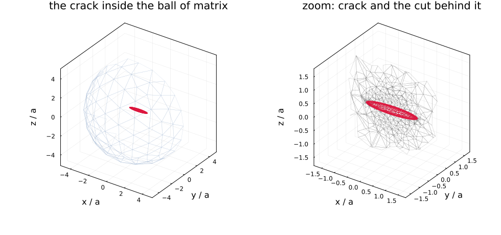
Left: the elliptical crack (red) suspended in the ball of matrix, whose far hemisphere is drawn in light blue — the crack is deliberately small, since
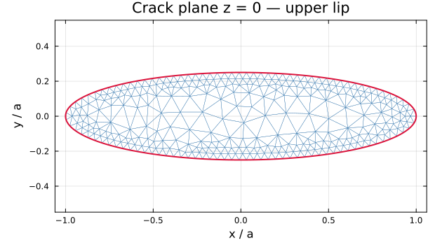
The upper lip seen from
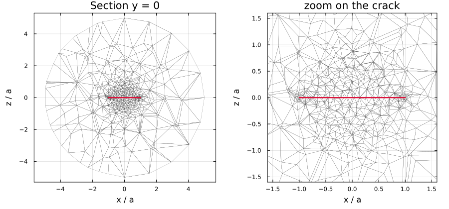
Two details are worth stating, because both cost real debugging time in the SifAniso study this is ported from:
the crack disc is
embeded in the ball, neverfragmented —fragmentwould cut the ball into two disjoint half-balls;gmsh's
Crackplugin duplicates the nodes of the crack front as well as those of the lips, in spite ofOpenBoundaryPhysicalGroup(still true in gmsh 4.15). Left alone the crack is effectively half an element larger than requested and the opening is overestimated by 10–20 %. The front is therefore welded back together after import, which is also why the tetrahedra stay geometrically straight:setOrder(2)runs after the plugin and curves the two lips' front edges differently, pulling the welded front apart again at the mid-side nodes.
Straight tetrahedra with a P2 displacement field, then — subparametric, and capped at P2 for the reason listed above.
A sphere with an off-center core
FEExcenteredSphere is the heterogeneous case, and it enters through gate B: being internally heterogeneous it has no Hill tensor, so it supplies both localization tensors directly. Its constituents live in the geometry object, core first then shell, and the Dict handed to add_phase! is a placeholder the kernel ignores.
C_core, C_shell = iso_stiffness(20.0, 12.0), iso_stiffness(6.0, 4.0)
incl = FEExcenteredSphere(1.0, (C_core, C_shell);
                          core_fraction = 0.5, eccentricity = 0.4)
A, B = fe_axi_localization(incl, C₀)          # both tensors, one solve
eccentricity is normalized by the largest offset that keeps the core inside, so it runs over core_fraction is the core's volume fraction within the inclusion. Because the geometry is axisymmetric, the cell is meshed in the meridian half-plane and the azimuthal dependence is carried by Fourier modes — a two-dimensional mesh for a three-dimensional answer. See FEAxiMeshOptions for the knobs and A recycled-concrete aggregate for the worked application, where the same correction is used in its general polarization-fixed-point form.
A superspherical or superspheroidal cavity
FESupershapePore is the non-ellipsoidal case, and the only one of the three that serves both physics from one object and one mesh. The shape comes from Supersphere or Superspheroid, and the exponent is
pore = FESupershapePore(Supersphere(1.0, 0.6);
                        opts = FECellMeshOptions(; level = 3, radius_ratio = 3.0))

rve = RVE()
add_phase!(rve, :m, Ellipsoid(1.0), Dict(:C => C₀, :K => K₀); fraction = :rest)
add_phase!(rve, :pores, pore, Dict(:C => C₀, :K => K₀); fraction = 0.05)
homogenize(rve, MoriTanaka(), :C)      # and :K, on the same mesh
The phase property is a placeholder and is ignored — see the cavity paragraph under Adding your own morphology above — so pass the matrix's own stiffness and nothing is lost. The same object answers from a network instead of a mesh when one is handed to it, FESupershapePore(shape; elastic = s), with everything else unchanged; that is the only way to differentiate the response with respect to
Keyword of FECellMeshOptions | Default | Meaning |
|---|---|---|
radius_ratio | 4.0 | outer radius over the shape's bounding radius |
level | 4 | inclusion surface subdivision: |
outer_level | 3 | outer sphere subdivision — not a free knob, see below |
relax | 60 | tangential relaxation sweeps on the inclusion surface |
octant | false | mesh one eighth of the cell — see below |
max_dofs, min_free_gb | 200_000, 6.0 | refuse a solve this machine cannot afford |
Five things about this cell are worth knowing before turning the knobs.
octant = true meshes one eighth of it, and the answer is the same. The condition is that the three coordinate planes be mirror planes of the shape — has_coordinate_mirrors, weaker than cubic symmetry, and true of both families here. It is worth a factor of eight in degrees of freedom and more in factorization cost: a concave shape at
Two consequences worth expecting. The stiffness is assembled once but factorized four times in elasticity and three in transport, one per parity class of the load cases — on a matrix eight times smaller, so the cost still falls sharply. And the couplings that symmetry forbids come out exactly zero instead of as mesh noise: the full cell finds the normal-to-shear block of
radius_ratio multiplies the bounding radius, not
outer_level is not a resolution trade-off. At outer_level = 2 the outer boundary carries 128 curved triangles, which does not resolve the
The boundary is curved, and it matters by a factor of about 16 in cost. setOrder(2) puts every mid-edge node at the midpoint of a straight segment — it cannot do better, the surface having been handed to gmsh as a discrete entity — so those nodes are pushed radially onto the exact shape afterwards, taking the geometry error from fe_cell_mesh_report reports three volumes so the gain is visible: for a sphere at level 2 the flat triangulation is off by 8.5 %, the curved boundary the solve actually sees by 0.23 %.
A strongly concave shape makes that snapping back off, and refining does not fix it. At a conical point the curvature is unbounded, so the nodes nearest it must stay short of the exact surface or they invert a neighboring element. The report's limited count says how many did. It grows with refinement — 6 nodes at level 2, 37 at level 3, 73 at level 4 for
A superspheroidal cavity, in two dimensions
FEAxiSupershapePore solves the axisymmetric member of the same shape family, and it is the cheapest inclusion in the package: the fields of a solid of revolution separate into Fourier modes in the azimuth, so each mode is a two-dimensional problem on the meridian half-plane.
pore = FEAxiSupershapePore(Superspheroid(1.0, 2.0, 0.7);
                           opts = FEAxiMeshOptions(; nradial = 24, radius_ratio = 6.0))
Everything downstream is unchanged — the same gate B, the same exactly-zero stress side, the same Dict placeholder for the phase property. What differs is what you get for the cost:
the answer is transversely isotropic, five constants in elasticity and two in transport, and the mode count delivers exactly that: a
at any refinement, being a structural identity of the class rather than a converged result; conduction on a sphere is exact to
Three things to know before turning the knobs. radius_ratio multiplies the bounding radius, as for the three-dimensional cell, so an elongated shape does not end up with its boundary at nprofile sets how finely it is sampled, tip_refine how much the elements shrink at the equatorial crease and the poles — because a concave superspheroid closes at the equator as a wedge whose half-gap is a fraction of a percent of nradial past 20 changes little, while going from fe_axi_pore_breakdown returns the uncorrected answer beside the corrected one, which is how to see that.
The derivation is in the pore declination; the comparison against the literature is in concave pores.
An N-layer spheroid, and the two exact families that check it
FEAxiLayeredSpheroid solves N nested coaxial spheroids in an isotropic matrix. Layers are given by their semi-axes, per layer, ascending — the same (axis_radii, disk_radii) pair LayeredSpheroid takes, in the same order — so one description builds the finite-element object and the analytic one:
ar, dr = confocal_layer_radii(2.0, 1.0, (0.3, 0.7))   # ω = 2, core 30 % of the volume
K = (TensISO{3}(5.0), TensISO{3}(2.0))
fe  = FEAxiLayeredSpheroid(ar, dr, K)
ana = LayeredSpheroid(ar, dr, K)                      # the same body, in closed form
Nothing in the finite-element type knows what confocal means, and that is the design: handed confocal_layer_radii it is the body the closed form solves, handed anything else it is a nest no closed form covers.
# An oblate core inside a prolate shell. Nested, axisymmetric, and outside every
# confocal family — which is the case the finite elements exist for.
FEAxiLayeredSpheroid((0.4, 1.4), (0.9, 1.0), K)
Nesting is checked at construction by check_nested_spheroids: two coaxial concentric ellipses are nested if and only if both semi-axes grow outwards, so it is two comparisons per layer. Worth doing rather than trusting — a violation is not a wrong answer but a self-intersecting geometry that gmsh rejects from inside its own pipeline, naming neither the layer nor the semi-axis.
What it is checked against. The space of nested spheroids is crossed by two independent exact families, meeting only at the equal-radii sphere:
| slice | closed form | agreement |
|---|---|---|
| confocal, prolate | LayeredSpheroid | 3\times10^{-5} |
| confocal, oblate | LayeredSpheroid | 2\times10^{-4} |
| concentric spheres, free radii | LayeredSphere | 1\times10^{-4} |
| equal moduli | the homogeneous spheroid's Hill tensor | 3\times10^{-5} |
Both branches of the confocal family are exercised deliberately: the oblate one runs the analytic computation in complex arithmetic, through the substitution
Off those slices the guarantees are each layer's meshed volume against the closed form
What is not implemented is the imperfect interface. The axisymmetric formulation has no displacement- or temperature-jump term at all — the only jump in the package is the three-dimensional crack's — so a spring, membrane, Kapitza or surface-conductive layer is refused by name at construction rather than accepted and ignored.
Being heterogeneous, the inclusion enters through gate B with both localization tensors, measured on the same solve: the stress side is not Voigt and Reuss work because the internal volume fractions are a closed form of the semi-axes, and layer_fractions returns them.
Morphologies still to come
Named here so that the boundary of what exists is explicit:
an anisotropic reference medium, which needs a Green-gradient model (Pan–Chou or Barnett–Willis) in place of the closed-form Kelvin dipole. This single restriction is what forces
IsoSymmetrize()under every iterative scheme;more than one inclusion, or a non-spherical envelope, in the axisymmetric cell;
transport for the crack: the elliptical-crack driver solves elasticity only, and the conduction problem would need its own resolution;
solid supershape inclusions. The cell is set up for a cavity: it meshes the matrix shell alone and leaves the inclusion boundary free, which is what makes the stress-side localization exactly zero. A solid inclusion would have to be meshed too, and would enter through gate B with two measured tensors, as the off-center core does;
These are tracked in the roadmap.
This page is static
Nothing here is computed at documentation-build time. The figures and the numbers are produced once by scripts/fe/make_doc_figures.jl and committed; the live demonstrations are scripts/81_fe_crack_eshelby.jl and scripts/82_fe_crack_schemes.jl.
Reproducing this page
julia scripts/fe/make_doc_figures.jl     # figures + docs/src/assets/fe/results.md.in
julia scripts/81_fe_crack_eshelby.jl     # the validation, live
julia scripts/82_fe_crack_schemes.jl     # the crack inside the schemes
See also
Custom inclusions — the contract these implement, and its three entry gates.
Adding a new inclusion — the full developer contract.
Neural-surrogate inclusions — how to make one of these solves cheap, and differentiable.
A recycled-concrete aggregate — the axisymmetric case, worked end to end.