📐
Theory
The Eshelby/Hill chain in the order it is built, then the ways it is generalized — richer patterns, conductivity, viscoelasticity, periodicity, N-body.
One Eshelby chain — Hill tensor, localization, scheme — generalized one direction at a time, in pure Julia and differentiable throughout.

Given a reference medium and an inclusion shape, MeanFieldHomogenization builds the Hill polarization tensor
That chain is the whole library. Everything else is the chain generalized in one direction at a time: a richer morphological pattern in place of the ellipsoid, a degenerate one for cracks, a different physics for transport, a different time dependence for viscoelasticity, a periodic problem for the multilayer, and no one-site assumption at all for the N-body schemes. The reading path takes them in that order.
MeanFieldHomogenization is a pure-Julia reimplementation of the Eshelby/Hill machinery of the Echoes C++/Python codebase; see From Echoes to MeanFieldHomogenization for the translation guide.
A porous solid, and every scheme the package ships, against the bounds that frame them. The void is given a small but non-zero stiffness, which is what lets the self-consistent branch stay on the physical solution:
using MeanFieldHomogenization, TensND, Plots
gr()  # headless backend; GKSwstype is set to "100" in make.jl

C_solid = iso_stiffness(90.0, 30.0)     # GPa
C_void  = iso_stiffness(0.01, 0.005)

function bulk(f, scheme)
    r = RVE()
    add_phase!(r, :M, Ellipsoid(1.0), Dict(:C => C_solid); fraction = :rest)
    f > 0 && add_phase!(r, :V, Ellipsoid(1.0), Dict(:C => C_void); fraction = f)
    return first(k_mu(homogenize(r, scheme, :C)))
end

fs = range(0.0, 0.5; length = 61)
schemes = ("Voigt" => Voigt(),
           "Reuss" => Reuss(),
           "Mori-Tanaka" => MoriTanaka(),
           "Dilute (dual)" => DiluteDual(),
           "Self-consistent" => AsymmetricSelfConsistent(; abstol = 1.0e-10,
                                                           maxiters = 200,
                                                           select_best = true),
           "Differential" => DifferentialScheme(; nsteps = 100))

plt = plot(; xlabel = "porosity f", ylabel = "effective bulk modulus k [GPa]",
             legend = :topright, framestyle = :box, size = (760, 470))
for (name, s) in schemes
    plot!(plt, fs, [bulk(f, s) for f in fs]; label = name, lw = 2)
end
plt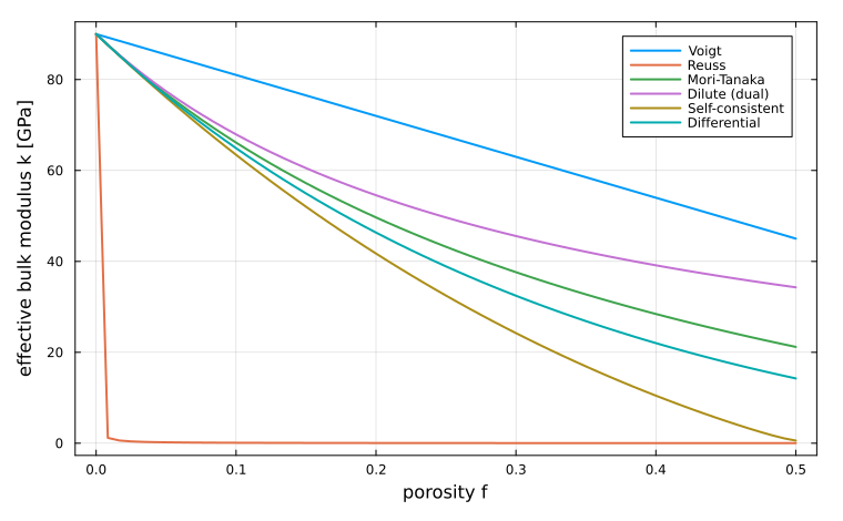
Voigt and Reuss bracket the others; the three estimates between them differ by how much of the load each void is assumed to see. Porous materials works through why the standard self-consistent scheme fails on this problem and what replaces it.