Nanocomposites: the equivalent particle

When the interface energy is of the same order as the bulk energy — the nanocomposite regime — the stress vector is discontinuous across a particle boundary and the polarization field of the Lippmann-Schwinger equation acquires a singular part carried by that boundary.

[35] show that averaging this singular part over the particle turns it into an ordinary stiffness,

after which the strain concentration rule keeps its classical form. No new scheme is needed: the equivalent particle drops into Mori-Tanaka — or any other estimate of the package — unchanged.

Two consequences run through everything below: scales as 1/size, so the stiffening is a genuine size effect; and for a spheroid it is transversely isotropic about the symmetry axis, hence carried exactly by five Walpole coefficients.

julia

using MeanFieldHomogenization
using TensND
using Printf
using Plots
gr()

default(; left_margin = 5Plots.mm, bottom_margin = 5Plots.mm)

§1 The interface stiffness across aspect ratios

κs and μs are the surface bulk and shear moduli, with the dimension of a stiffness times a length. The values used here are those the paper identifies for graphene sheets from the data of Alzebdeh (2012).

julia

κs, μs = 64.0, 51.3          ## Pa·m, graphene (paper, Fig. 3)
a = 1.0                      ## in-plane semi-axis

# Aspect ratio X = c/a: oblate below 1, prolate above.
function Cint_components(X)
    ell = X < 1 ? Ellipsoid(a, a, X * a) : (X > 1 ? Ellipsoid(X * a, a, a) : Ellipsoid(a))
    A = get_array(surface_stiffness(ell, κs, μs))
    # Read in the frame of the symmetry axis: e₃ for oblate/sphere, e₁ for prolate.
    return X > 1 ? (A[2, 2, 2, 2], A[1, 1, 1, 1], A[2, 2, 3, 3], A[1, 2, 1, 2]) :
        (A[1, 1, 1, 1], A[3, 3, 3, 3], A[1, 1, 2, 2], A[1, 3, 1, 3])
end

Xs = 10.0 .^ range(-2, 2; length = 121)
Ct, Cax, Ctt, Cs = Float64[], Float64[], Float64[], Float64[]
for X in Xs
    t, ax, tt, s = Cint_components(X)
    push!(Ct, t); push!(Cax, ax); push!(Ctt, tt); push!(Cs, s)
end

p1 = plot(
    Xs, Ct; xscale = :log10, yscale = :log10,
    xlabel = "aspect ratio X = c/a", ylabel = "component of ℂ^int  [Pa]",
    title = "Interface stiffness of a spheroid", label = "transverse (1111)",
    legend = :bottomleft, lw = 2
)
plot!(p1, Xs, Cax; label = "axial (3333)", lw = 2)
plot!(p1, Xs, abs.(Ctt); label = "|cross (1122)|", lw = 2, ls = :dash)
plot!(p1, Xs, Cs; label = "axial shear (1313)", lw = 2, ls = :dot)
vline!(p1, [1.0]; color = :black, ls = :dashdot, label = "sphere")
p1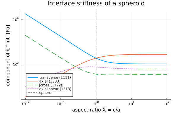

§2 The three limiting cases of the paper

The closed form has a removable singularity at X = 1 (both terms diverge as (X²-1)⁻² and cancel); the implementation switches to a series there, so the spherical case is exact rather than merely close.

julia

println("Spherical limit X = 1, closed form:")
R = 1.0
A = get_array(surface_stiffness(Ellipsoid(R), κs, μs))
@printf "  C_1111 = %.6f   vs  8(κs+μs)/(5R) = %.6f\n" A[1, 1, 1, 1] 8 * (κs + μs) / (5R)
@printf "  C_1122 = %.6f   vs  2(3κs-2μs)/(5R) = %.6f\n" A[1, 1, 2, 2] 2 * (3κs - 2μs) / (5R)
@printf "  C_1313 = %.6f   vs  (κs+6μs)/(5R) = %.6f\n" A[1, 3, 1, 3] (κs + 6μs) / (5R)

println("\nAsymptotic oblate limit X → 0 (platelet):")
c = 1.0e-6
B = get_array(surface_stiffness(Ellipsoid(1.0, 1.0, c), κs, μs))
@printf "  c·C_1111 = %.6f   vs  3(κs+μs)/2 = %.6f\n" c * B[1, 1, 1, 1] 3 * (κs + μs) / 2
@printf "  c·C_1122 = %.6f   vs  3(κs-μs)/2 = %.6f\n" c * B[1, 1, 2, 2] 3 * (κs - μs) / 2
@printf "  c·C_1212 = %.6f   vs  3μs/2      = %.6f\n" c * B[1, 2, 1, 2] 3μs / 2
@printf "  c·C_3333 = %.3e  (vanishes: a platelet stiffens only in its plane)\n" c * B[3, 3, 3, 3]

println("\nAsymptotic prolate limit X → ∞ (nanofiber):")
D = get_array(surface_stiffness(Ellipsoid(1.0e6, 1.0, 1.0), κs, μs))
@printf "  axial   C = %.6f   vs  3π(κs+μs)/(4a) = %.6f\n" D[1, 1, 1, 1] 3π * (κs + μs) / (4a)
@printf "  C_1111/C_1122 = %.6f   vs  3 (compared with atomistics in the paper)\n" D[2, 2, 2, 2] / D[2, 2, 3, 3]

Spherical limit X = 1, closed form:
  C_1111 = 184.480000   vs  8(κs+μs)/(5R) = 184.480000
  C_1122 = 35.760000   vs  2(3κs-2μs)/(5R) = 35.760000
  C_1313 = 74.360000   vs  (κs+6μs)/(5R) = 74.360000

Asymptotic oblate limit X → 0 (platelet):
  c·C_1111 = 172.950000   vs  3(κs+μs)/2 = 172.950000
  c·C_1122 = 19.050000   vs  3(κs-μs)/2 = 19.050000
  c·C_1212 = 76.950000   vs  3μs/2      = 76.950000
  c·C_3333 = 3.459e-10  (vanishes: a platelet stiffens only in its plane)

Asymptotic prolate limit X → ∞ (nanofiber):
  axial   C = 271.669225   vs  3π(κs+μs)/(4a) = 271.669225
  C_1111/C_1122 = 3.000000   vs  3 (compared with atomistics in the paper)

§3 The size effect

under a homothety of ratio under a homothety, so the interface matters for small particles and disappears for large ones. Feeding the equivalent particle to Mori-Tanaka makes that visible directly on the effective moduli.

julia

k_m, μ_m = 30.0, 20.0                       ## a polymer-like matrix, GPa
C_m = TensISO{3}(3k_m, 2μ_m)
C_i = TensISO{3}(3 * 120.0, 2 * 80.0)       ## a stiff filler
f = 0.15

function mt_with_interface(radius; with_interface = true)
    sph = Ellipsoid(radius)
    C_eq = with_interface ? equivalent_particle(C_i, sph, κs * 1.0e-9, μs * 1.0e-9) : C_i
    rve = RVE()
    add_phase!(rve, :M, Ellipsoid(1.0), Dict(:C => C_m); fraction = :rest)
    add_phase!(rve, :nano, sph, Dict(:C => C_eq); fraction = f)
    return get_array(homogenize(rve, MoriTanaka(), :C))[1, 2, 1, 2]
end

radii = 10.0 .^ range(-9, -6; length = 60)       ## 1 nm to 1 μm
μ_nano = [mt_with_interface(r) for r in radii]
μ_bulk = mt_with_interface(1.0; with_interface = false)

@printf "\nMori-Tanaka with the equivalent particle, f = %.2f:\n" f
for r in (1.0e-9, 5.0e-9, 2.0e-8, 1.0e-7)
    @printf "  radius %6.1f nm :  μ_eff = %.4f GPa   (+%.1f %% vs no interface)\n" r * 1.0e9 mt_with_interface(r) 100 * (mt_with_interface(r) / μ_bulk - 1)
end

p2 = plot(
    radii .* 1.0e9, μ_nano; xscale = :log10,
    xlabel = "particle radius [nm]", ylabel = "μ_eff  [GPa]",
    title = "Size effect through the equivalent particle",
    label = "with interface", lw = 2, legend = :topright
)
hline!(p2, [μ_bulk]; ls = :dash, label = "no interface")
p2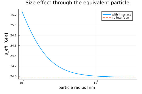

§4 Shape at fixed volume fraction

Platelets and fibers do not stiffen the same way: the oblate limit concentrates the interface effect in the plane of the particle, the prolate one spreads it over every component.

julia

Xs2 = 10.0 .^ range(-1.5, 1.5; length = 40)
μ_shape = Float64[]
for X in Xs2
    # Fixed particle volume, varying aspect ratio.
    a0 = (1.0e-8^3 / X)^(1 / 3)
    ell = X < 1 ? Ellipsoid(a0, a0, X * a0) : Ellipsoid(X * a0, a0, a0)
    C_eq = equivalent_particle(C_i, ell, κs * 1.0e-9, μs * 1.0e-9)
    rve = RVE()
    add_phase!(rve, :M, Ellipsoid(1.0), Dict(:C => C_m); fraction = :rest)
    add_phase!(rve, :nano, ell, Dict(:C => C_eq); fraction = f, symmetrize = :iso)
    push!(μ_shape, get_array(homogenize(rve, MoriTanaka(), :C))[1, 2, 1, 2])
end

p3 = plot(
    Xs2, μ_shape; xscale = :log10,
    xlabel = "aspect ratio X = c/a", ylabel = "μ_eff  [GPa]",
    title = "Orientation-averaged, fixed volume and fraction",
    label = "with interface", lw = 2, legend = :bottomright
)
vline!(p3, [1.0]; color = :black, ls = :dashdot, label = "sphere")
p3

p_full = plot(p1, p2, p3; layout = (1, 3), left_margin = 8Plots.mm, bottom_margin = 8Plots.mm,
    size = (1500, 520), titlefontsize = 9)
p_full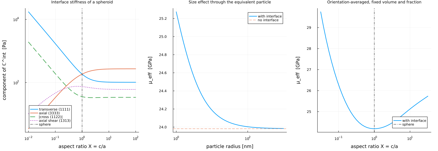

This page was generated using Literate.jl.

Nanocomposites: the equivalent particle ​

§1 The interface stiffness across aspect ratios ​

§2 The three limiting cases of the paper ​

§3 The size effect ​

§4 Shape at fixed volume fraction ​

Nanocomposites: the equivalent particle

§1 The interface stiffness across aspect ratios

§2 The three limiting cases of the paper

§3 The size effect

§4 Shape at fixed volume fraction