MFH Studio: building scripts graphically

MFH Studio is a local web interface that builds MeanFieldHomogenization scripts. It draws the shape of the phase being edited, runs the model, and — the part that makes it safe to use on existing work — reads a script back and preserves everything it does not recognize.

The script stays the deliverable. The studio is a way of writing one, not a format to be locked into.

Starting the studio

From a Julia session with MeanFieldHomogenization loaded — the studio ships with the checkout you develop:

using MeanFieldHomogenization
mfhstudio()                  # starts the server and opens a browser
mfhstudio(port = 9000)       # pick a different port
mfhstudio(no_browser = true) # stay in the terminal
mfhstudio(check = true)      # verify the Julia side and exit

MeanFieldHomogenization.mfhstudio Function

mfhstudio(; host="127.0.0.1", port=8765, no_browser=false,
          project=nothing, julia=nothing, python=nothing,
          check=false, wait=true)

Start MFH Studio, the graphical builder for MeanFieldHomogenization scripts, and block until it stops (press Ctrl-C in the REPL — the SIGINT reaches the server in the same process group and shuts it down cleanly). With wait = false, spawn the server and return its Process handle immediately, leaving the REPL free.

The server is the Python app under tools/mfhstudio of the MeanFieldHomogenization checkout, run as python -m mfhstudio. Python 3.10+ (standard library only) must be on PATH, or pointed at with the python keyword argument or the MFHSTUDIO_PYTHON environment variable. The first interpreter on PATH that can actually import the studio is used, which on Windows means py -3 is tried after python and python3 — those two are often a Store stub or an MSYS2 build there.

Arguments

• host/port — where to bind; the printed URL is http://host:port/. Pick a different port when the default 8765 is taken.

• no_browser — start without asking the browser to open.

• project — Julia environment for the sidecar: a directory, or @name for a shared one. Defaults to the MeanFieldHomogenization checkout (as the Python app does), honoring MFHSTUDIO_PROJECT.

• julia — Julia executable for the sidecar if it is not on PATH (the JULIA environment variable is honored too).

• check — verify the Julia side and exit instead of serving.

• wait — block until the server stops (default) or return its process handle.

Examples

using MeanFieldHomogenization
mfhstudio()                  # http://127.0.0.1:8765, opens a browser
mfhstudio(port = 9000)       # pick a different port
mfhstudio(no_browser = true) # stay in the terminal
p = mfhstudio(wait = false)  # keep the REPL; later `wait(p)` or `kill(p)`

mfhstudio blocks the REPL, like Pluto.run(), until the studio stops: Ctrl-C in the REPL shuts the server and its Julia sidecar down cleanly. Pass wait = false to keep working while the studio runs — it returns the process handle, and wait(p) / kill(p) take it down again. host, port, project, julia and python map onto the Python app's command-line options below; project = "@mfhstudio" uses a shared environment, julia = ... / python = ... point at a specific executable (or set the MFHSTUDIO_PROJECT / MFHSTUDIO_PYTHON environment variables).

The same tool starts from a shell — Python 3.10+ underneath, standard library only:

cd tools/mfhstudio
python3 -m mfhstudio                # starts the server and opens a browser
python3 -m mfhstudio --port 9000    # pick the port
python3 -m mfhstudio --no-browser   # stay in the terminal
python3 -m mfhstudio --check        # verify the Julia side and exit

On Windows, python -m mfhstudio.

It needs Python 3.10+ (standard library only) and a julia on PATH able to load MeanFieldHomogenization. Loading the package takes about ten seconds, paid once when the interface starts; the badge in the top-right turns green when it is ready. On a fresh checkout the sidecar instantiates the package environment first, which takes a few minutes once.

If Julia cannot start, the interface still comes up and says so in a banner: building and saving a script works, while the 3-D view, reading a script back and Run are off. --check diagnoses the Julia side without paying the load time, and is the right first command on a new machine.

One failure is worth knowing about. A development machine's local Manifest.toml — untracked, one per clone — may pin some dependencies to sibling checkouts (path = "../TensND.jl"), which only resolve when those siblings are there. If yours does and they are not, the studio does not need the clone's environment at all: MeanFieldHomogenization is registered in General, so a shared environment resolves everything from the registry.

using Pkg
Pkg.activate("mfhstudio", shared = true)
Pkg.add("MeanFieldHomogenization")

To run the studio against a clone you are editing rather than the released version, develop it into that same environment instead:

Pkg.develop(path = raw"<path to MeanFieldHomogenization.jl>")

Either way, start the studio against that shared environment — mfhstudio(project = "@mfhstudio"), or --project @mfhstudio from the shell. --check reads the manifest and names the missing checkouts itself.

Start here: the worked examples

The quickest way in is not to build a model but to open one. Open… starts in tools/mfhstudio/examples/, which holds ten small models covering most of what the interface can express:

file	what it shows
01_porous_schemes.jl	every scheme on one figure — where they agree, and where they fail
02_cracked_solid.jl	cracks entering with a density, and orientation averaging
03_coated_inclusion.jl	one inclusion with concentric shells
04_conductivity_fibers.jl	the same schemes answering a conduction problem
05_two_scales.jl	the multiscale seam, and a sweep reaching through it
06_laminate_basics.jl	the exact laminate; Backus, and both bounds saturating
07_laminate_interfaces.jl	an imperfect interface and the size effect it brings
08_laminate_multiscale.jl	a layer that is itself a homogenized cell
09_ageing_creep.jl	a viscoelastic phase, and the creep curve
10_sensitivities.jl	derivatives of the effective property, by autodiff

Each is a running script and a filled-in model: open one, change a number in the form, watch the Julia on the right follow, press Run. Each names the scripts/ demo it is drawn from, so the physics is one click away.

They are the studio's own output — generated by examples/build_examples.py from the same code generator that writes your scripts — which is why they reopen with every form filled in. The hand-written demos in scripts/ do not: they build their cells at top level, the way one writes Julia directly, and the studio preserves those verbatim rather than offering them for editing. Read scripts/ for the physics; open examples/ to turn the knobs.

The layout

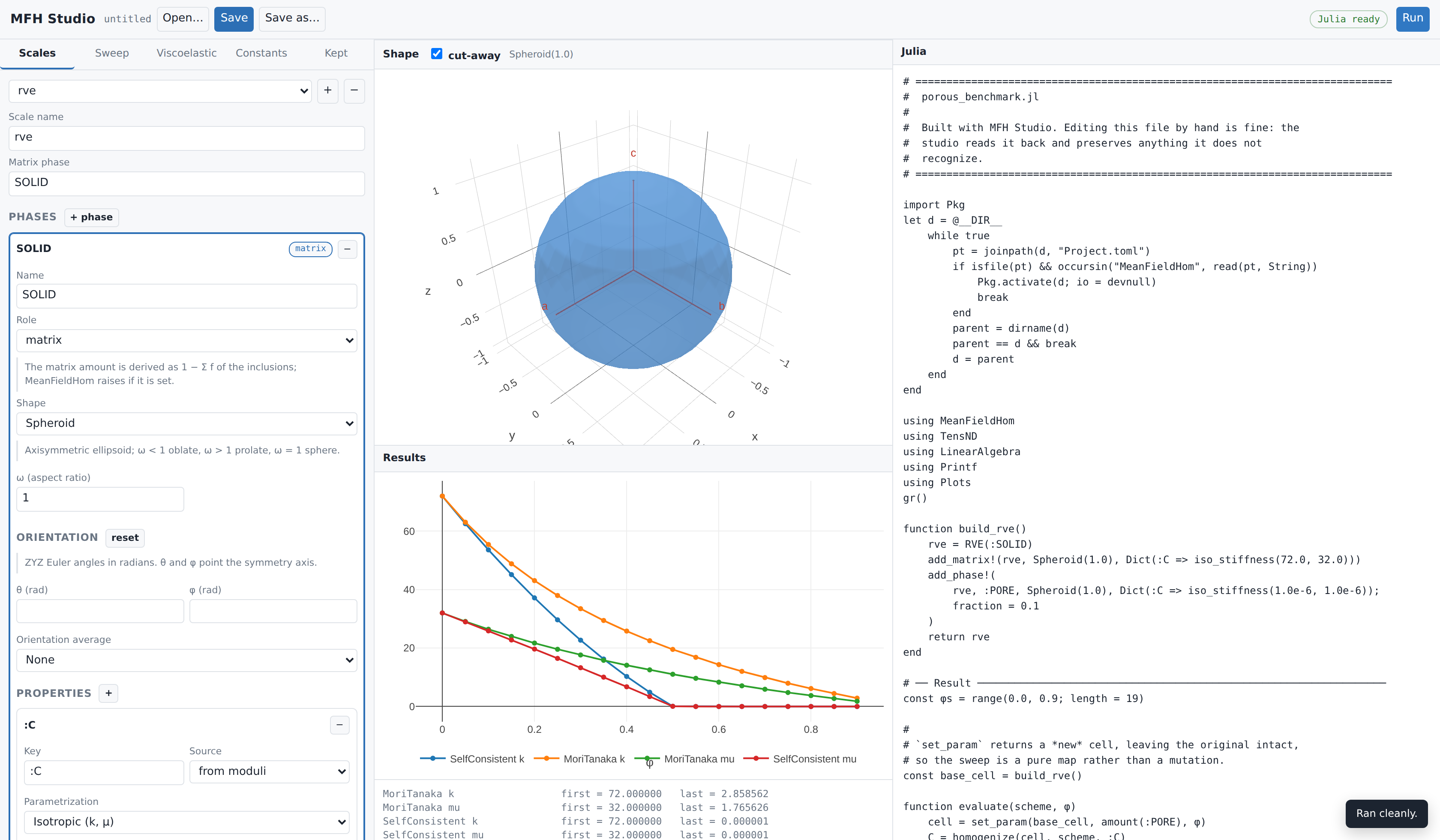
Three columns: the model on the left, the shape and the results in the middle, the Julia on the right. The script is regenerated on every edit, so what is displayed is exactly what Save writes.

Every boundary between panels is a drag handle — the two between the columns, and the ones between the graph, the 3-D view, the results and the output log. Double-click a handle to put that one back where it started. The sizes are remembered between sessions, per browser.

The Shape panel draws the geometry of the phase currently selected — a single inclusion, from its semi-axes and orientation. It is not a picture of the microstructure: mean-field homogenization never builds one, and nothing here places inclusions in a volume or shows how they are distributed. What the panel is good for is checking that the shape you described is the shape you meant.

The screenshot shows the porous benchmark after pressing Run — a solid matrix   with spherical pores swept over  . The numbers reproduce the Budiansky–O'Connell values captured from Echoes 1.0 (see From Echoes to MeanFieldHomogenization).

Two conventions the interface removes rather than documents:

• A phase whose amount is set to rest has no value field. MeanFieldHomogenization derives it as   and refuses to have it set, so offering the field would only invite an error.

• Moduli are entered as physical or and emitted through iso_stiffness. The raw TensISO{3} constructor, which takes , never appears.

Shapes that have one carry an Orientation block: ZYZ Euler angles in radians, as many as the shape admits — two for a spheroid or a penny crack, which only need their axis pointed, three for an ellipsoid or an elliptic crack. The field shows the degree equivalent beside the label, and the drawing follows, so a mis-typed angle is visible rather than hidden until the numbers come out wrong.

Solver options follow the scheme rather than homogenize, and the list offered for each scheme is read from the scheme itself — SelfConsistent shows abstol, reltol, maxiters, damping, select_best, verbose; DifferentialScheme shows nsteps and formulation. The interface cannot fall behind MeanFieldHomogenization because it never hard-codes that list.

The default shown beside each option is the one the scheme actually uses, and it is not the same for every scheme: the self-consistent solvers stop at abstol = 1e-12, reltol = 1e-8, while DifferentialScheme hands 1e-8 / 1e-6 to OrdinaryDiffEq. Overriding abstol alone rarely changes anything — see Solver tolerances.

Layered inclusions

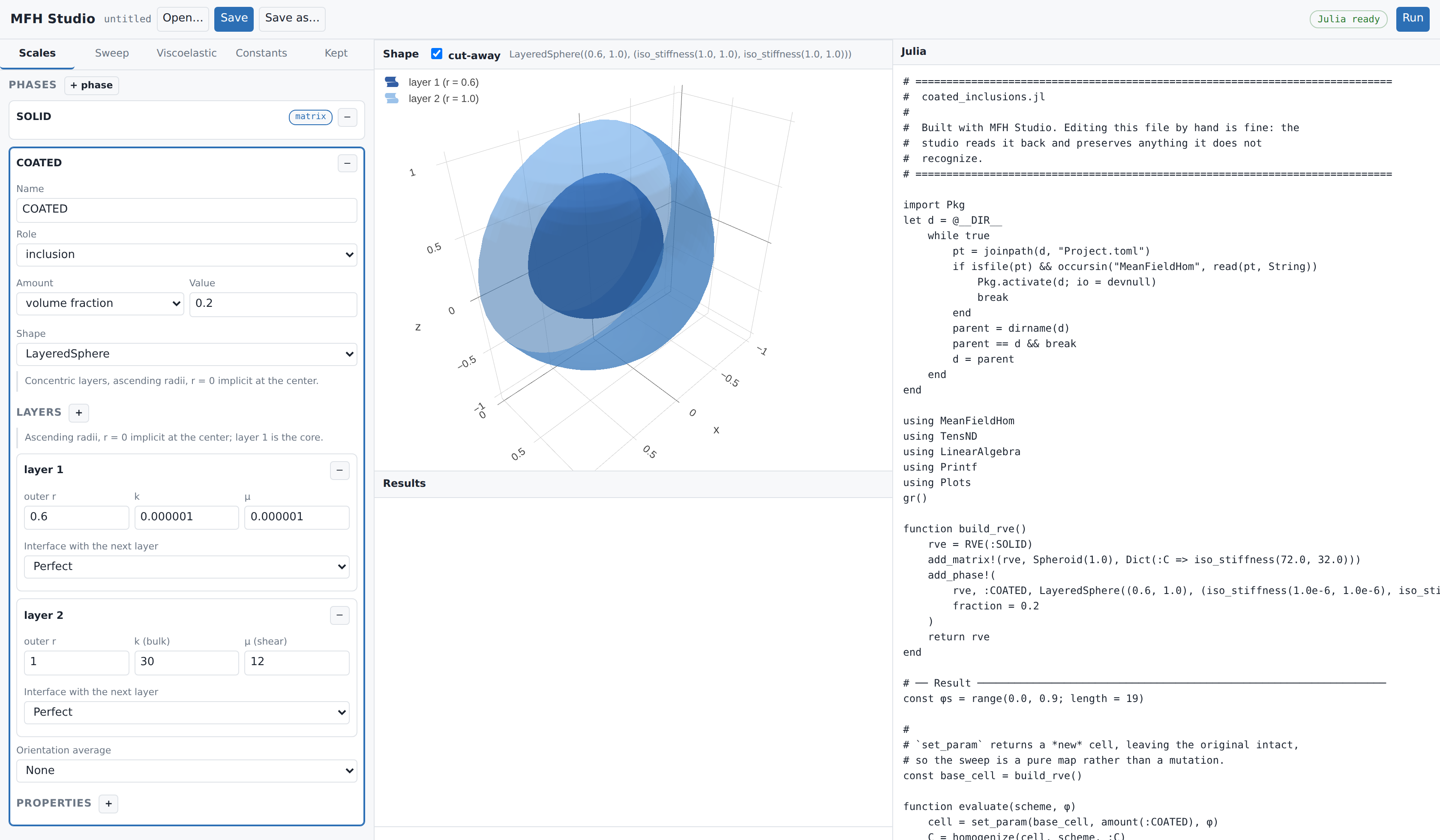
Choosing LayeredSphere turns the phase editor into a table of layers — outer radius, moduli, and the interface with the next layer (perfect, spring, membrane, Kapitza, surface-conductive). The 3-D view cuts the shells open, which is the only way a layered inclusion is readable at all: without the cut-away only the outermost shell is visible.

Radii are ascending with   implicit at the center, and layer 1 is the core — the same convention as LayeredSphere.

A LayeredSpheroid is described differently, because it must be confocal: every layer shares one focal distance, and radii entered one by one essentially never do. The form therefore asks for the outer aspect ratio, the outer semi-axis and a volume fraction per layer, and layered_spheroid_from_fractions solves for the confocal radii. It is a conduction geometry, so its layers carry a conductivity rather than moduli.

Laminates

Everything above describes an RVE: a matrix with inclusions dispersed in it, a random morphology that the mean-field schemes estimate. The Kind selector at the top of the Scales panel offers a second kind of cell.

A laminate is a periodic stack of parallel layers of common normal. It has no matrix, no reference medium and no auxiliary Eshelby problem — and its effective behavior is exact, not an estimate. It is the deterministic counterpart of the morphologies the rest of the interface describes.

Picking Laminate replaces the phase list with a stack:

• a stacking direction, given as ZYZ Euler angles — the form everything else in the interface is oriented with, so a stack reads in the same units as the anisotropic properties around it — or, for a script that states one, as a normal vector. The normal is the frame's third axis: θ tilts it away from e₃, φ turns it about e₃, and ψ spins the layer axes in the plane. Either way the canonical frame (no angles, or (0, 0, 1)) is where the kernel skips the frame rotation entirely and nothing is written into the script;

• a layer table, in stacking order, with ↑/↓ to reorder. Each layer carries a full property editor — so a layer can hold an anisotropic tensor, a viscoelastic law, or the effective property of another scale, exactly as a phase can;

• an interface on top of each layer, the last one closing the cell back onto the first by periodicity.

The 3-D view draws the stack itself rather than one member, because the geometry of a laminate is the stacking direction: there is no per-layer shape. The cut-away slices it so the cross-section — the only informative view of something unbounded in its own plane — faces you.

A cell, not an inclusion

A laminate cannot be put inside a matrix. Embedding one would need its Hill tensor, which is a different and open problem. It sits beside an RVE in the scale graph, and the two connect through the ordinary seam.

Layers are given either by volume fraction (summing to 1) or by absolute thickness, never a mix — MeanFieldHomogenization refuses that, and so does the form. The distinction is physical rather than cosmetic: with a perfect interface the answer depends on the fractions alone, but an imperfect one enters with weight , an interface density, so the absolute period carries a size effect. 07_laminate_interfaces.jl shows it: thickening the stack stiffens it.

Only three schemes apply, and the scheme list narrows to them as soon as the target cell is a laminate:

scheme	what it is
Laminated	the exact periodic solution
Voigt, Reuss	the bounds, which need no matrix phase

Asking for anything else is reported before the run rather than raised inside it. 06_laminate_basics.jl is worth opening for what it shows about those three: a laminate is exactly Reuss across the layers and exactly Voigt in their plane, at the same time.

Two parameters exist only here, and appear in the Sweep and Sensitivity lens lists when the target is a laminate:

• layer thickness — not the same as a volume fraction. Changing moves both and the period, so with an imperfect interface the thickness derivative also carries the size effect, which is usually what one wants;

• interface field — one scalar of one interface (, , , , the Kapitza resistance, the surface conductance). Interface sits on top of layer .

Conversely a laminate has no phase amount: AmountParameter raises on one and points at the thickness instead, so the interface offers the thickness and not the amount.

Sensitivities

The Sensitivity tab differentiates the effective property through the whole scheme, by forward-mode automatic differentiation — not by finite differences, so there is no step size to choose and no cancellation to worry about.

There is nothing new to learn: the parameter is the same lens the sweep uses, and the differentiated quantity is the same output the sweep plots. The point is the model itself — get_param reads it off the cell — so the amounts and moduli already entered in Scales are where the derivative is taken, and nothing is typed twice.

kind	parameters	result
derivative	exactly one
gradient	several	one number per parameter
jacobian	several	the whole effective tensor, flattened, against each parameter

gradient(cell, scheme, [amount(:PORE), property(:SOLID, :C, 1)];
         output = :C, indexer = C -> k_mu(best_fit_iso(C))[1])

The reporting projection sits inside the differentiated function, so what comes out is the derivative of the quantity actually reported. A jacobian extracts no scalar at all, which is also the way out when the result is not isotropic and k_mu therefore has no method for it.

The answer is a table in the output panel rather than a figure: a gradient is not a curve.

A sensitivity crosses scales like everything else — the nested lens composes through the seam, and the whole chain is differentiated in one pass.

Multiscale

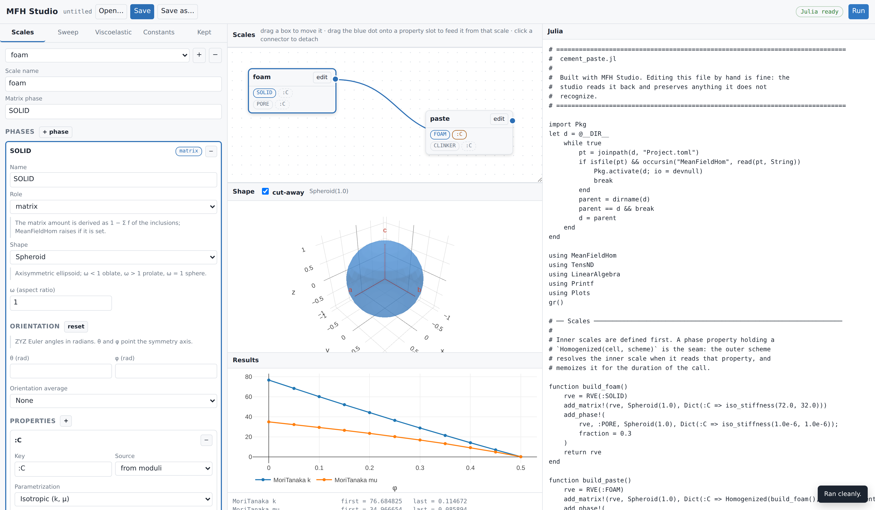
This is where the interface earns the most. MeanFieldHomogenization chains scales declaratively: a phase property may hold a Homogenized(inner_cell, scheme) instead of a tensor, and the outer scheme resolves the inner scale when it reads that key (see Multiscale models).

The Scales panel draws that graph. Each box is a scale; the blue dot on its right is its effective property; the dashed slots are the property keys of its phases. Dragging the dot onto a slot creates the seam — the connector appears and the Julia updates immediately. Clicking a connector detaches it.

The screenshot reproduces the foam/paste model of the multiscale manual: a foam homogenized self-consistently feeds the matrix of a paste containing clinker inclusions. The generated script emits build_foam() before build_paste(), because the graph is sorted topologically before writing.

A scale cannot feed itself: a connection that would close a cycle is refused when it is made, not when the script runs.

The sweep can cross scales too. The nested lens reaches through a seam into the inner cell, so sweeping the foam's porosity from the outer model is one lens rather than a hand-written closure:

cell = set_param(base_cell, nested(:FOAM, :C, amount(:PORE)), φ)

Not combinable with ageing viscoelasticity

An inner Homogenized cannot sit inside an ALV chain — the inner result would have to be re-expressible as a ViscoLaw. The interface refuses the combination instead of writing a script that fails at run time.

Choosing what to compute

Three tabs produce a result, and they are exclusive — a script has one Result section, so turning one on turns the others off:

tab	what it writes
Sweep	one point, or a curve over a lens
Sensitivity	derivatives, by autodiff
Viscoelastic	an ageing creep or relaxation curve

The Sweep tab decides the shape of the run.

One point homogenizes once with the amounts entered in Scales — the answer when you simply want the number for the fractions you typed. Sweep varies one lens over a range and draws the curve.

Either way the schemes are a list: adding a second one puts both on the same figure, which is usually the reason to draw one. Each carries its own solver options, and switching a scheme clears them, because they belong to the scheme that reads them — MoriTanaka(; verbose = false) is a MethodError, the singleton schemes taking no keywords at all.

The outputs are chosen too, and this matters more than it looks:

Output	Defined for
k, μ, E, ν	an isotropic result only
Kelvin-Mandel component KM[i,j]	any symmetry
tensor component C[i,j]	2nd-order properties (conduction)
tr/3	mean conductivity

Clip negative values to zero is the other reporting choice, and it belongs to the figure rather than to the physics. A scheme pushed outside its range returns negative moduli — Dilute does, well before   — and on a figure shared by several schemes that one curve sets the scale for all of them. scripts/28_porous_schemes.jl clips for exactly that reason, and 01_porous_schemes.jl reproduces it. Plotting a single scheme, leave it unticked: a negative modulus is then the useful signal that the estimate has stopped meaning anything.

k_mu has a method for TensISO (a TensND type) and nothing else. An oriented inclusion with no orientation average does not give an isotropic effective tensor, so asking for k there fails deep inside the run with a MethodError. The interface says so before you run: either pick a reporting projection, or plot components, which are defined whatever the symmetry.

Viscoelasticity

A phase becomes viscoelastic through its property, not through a separate panel: in Scales → Properties → Parametrization, choose Maxwell, a Kelvin chain, an elastic (Heaviside) phase, or a custom . The generated call uses MeanFieldHomogenization's own signatures — maxwell_iso(k, μ, η_k, η_μ) takes two relaxation times, kelvin_iso takes whole branch vectors.

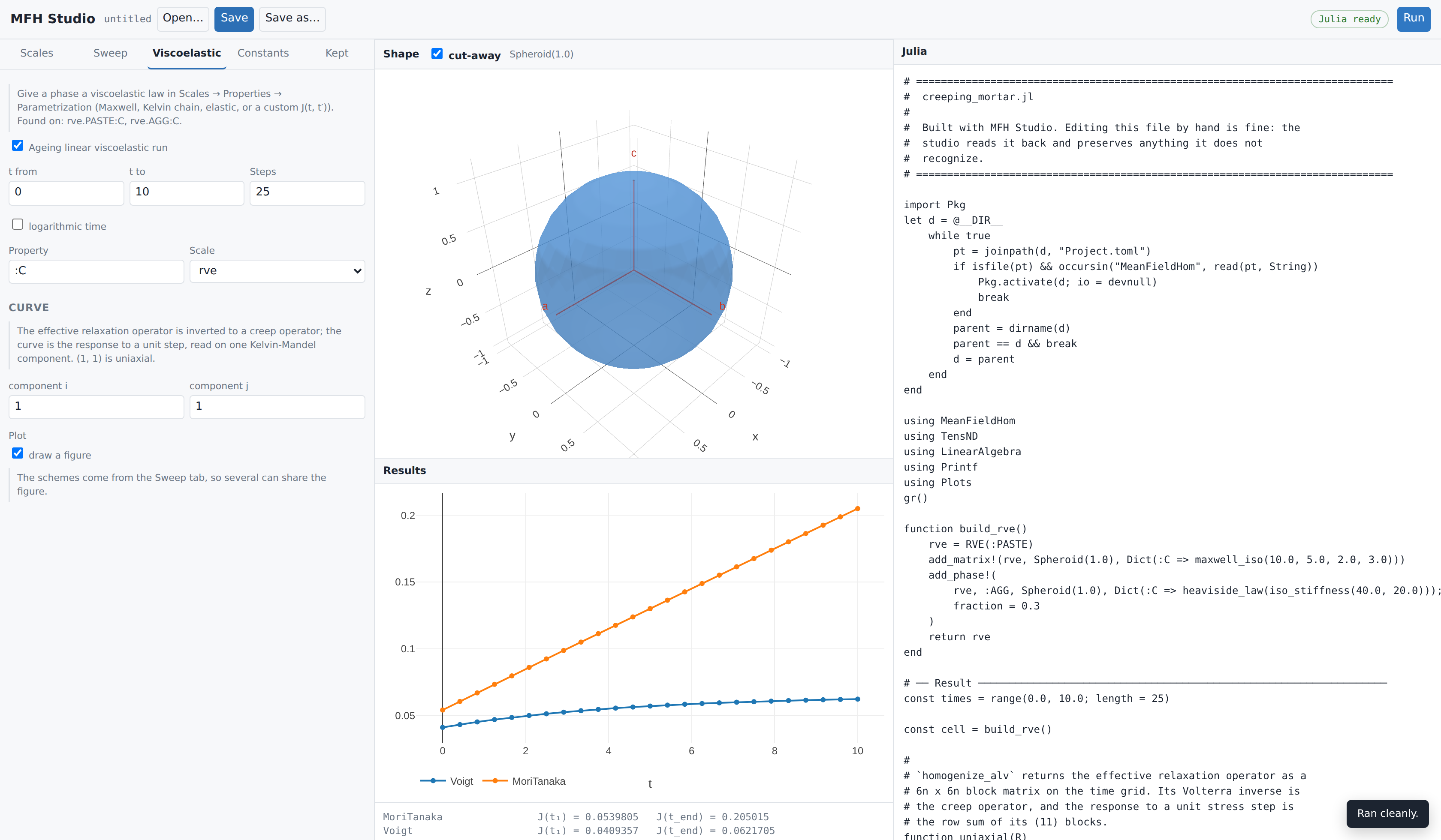
The Viscoelastic tab then only decides the time grid and the curve. It lists which phases carry a law, so a run with nothing to age says so rather than failing later. homogenize_alv returns the effective relaxation operator as a   block matrix; the curve is its Volterra inverse read on one Kelvin-Mandel component — (1, 1) is the uniaxial creep response, the extraction used in scripts/62_alv_schemes.jl.

Anisotropic properties

Conductivity comes in three forms: isotropic , transversely isotropic , and orthotropic . Stiffness offers isotropic or , transversely isotropic Hoenig parameters, and the nine orthotropic constants. Anything else is typed as a Julia expression, which the generator passes through untouched.

The frame the constants are written in

An anisotropic tensor means nothing without its frame, so every anisotropic form carries its own Orientation block of ZYZ Euler angles. It is not the shape's orientation: a tilted fiber made of an untilted material and an untilted fiber made of a tilted material are different materials, and the two angle sets are stored and emitted separately.

What the angles produce depends on the symmetry class. A transversely isotropic tensor carries an axis rather than a basis — is irrelevant, the transverse plane being isotropic — so the studio emits the third vector of the frame:

hoenig_stiffness(30.0, 0.3, 0.2, 0.25, 0.5, vecbasis(RotatedBasis(π/4, 0.7, 0.0))[:, 3])
TensTI{2}(1.0, 5.0, vecbasis(RotatedBasis(π/4, 0.7, 0.0))[:, 3])

An orthotropic tensor needs all three directions, and takes the basis itself. Tens(A, basis) stores A as the components in that basis, which is what "diagonal in the material frame" means:

TensOrtho(120.0, 90.0, 70.0, 40.0, 35.0, 30.0, 25.0, 22.0, 20.0, RotatedBasis(0.3, π/3, 0.0))
Tens([1.0 0.0 0.0; 0.0 2.0 0.0; 0.0 0.0 5.0], RotatedBasis(0.3, π/3, 0.0))

Angles are radians, and the field accepts arithmetic: π/4, 2pi/3 and plain decimals all work, an expression reaching the script as written rather than as its seventeen-digit decimal. The degree equivalent is shown beside each field.

The isotropic point of the Hoenig parametrization

  together with   and   is not a transversely isotropic material: it is the isotropic one, written in a transversely isotropic type. The axis then carries no information, and the schemes have a degenerate reference to work from. The defaults are away from that corner for this reason.

Opening an Echoes script

Open accepts a .py as well as a .jl. Picking a Python file makes the studio translate it with echoes2mfh, ask where the Julia should go, write it, and open the result — one action rather than a separate convert button, because the extension already says which of the two is happening.

The translator's findings come back with it. A script it could not translate whole reports how many constructs it refused, and each one sits in the written script as an UNTRANSLATED block that raises at run time, so a half-translated model cannot quietly produce numbers.

Reading an existing script

Open… browses the server's own filesystem — with shortcuts to examples/, scripts/, the package root and your home directory — rather than using the browser's file input. The browser never reveals a real path, and a path is exactly what saving back to the same file needs; listing server-side also keeps the picker correct when the studio runs on a remote machine. Save writes to the current file, Save as… asks for a new one.

Reading a .jl file back, two things can happen.

A script the studio wrote carries its model in a trailing comment block and reopens exactly. Any other script — a hand-written demo from scripts/, an echoes2mfh translation — is parsed by the Julia side using Meta.parse, the real parser, and matched against the vocabulary the generator emits: a builder function per scale, filled with add_phase! for an RVE or with add_layer! for a laminate. Code outside that vocabulary — including a cell assembled at top level rather than inside a builder — is not claimed.

Everything else is kept verbatim. It appears under the Kept tab, read only, and is written back byte for byte. Editing the model never rewrites it.

The rule is stricter than "parse what you can": a construct is only claimed when the studio can prove it reproduces it. Before accepting a builder, the reader renders it exactly as it would be saved and compares with the source; if the two differ, the original text is kept and the reason is shown. That is why a demo like scripts/28_porous_schemes.jl, whose builder takes typed and keyword arguments the model does not represent, opens without being damaged.

Constants behave the same way: one read from a file keeps its original text — multi-line layout included — until you actually edit it.

Across the 60 demo scripts in scripts/ and the translations produced by echoes2mfh, opening and writing back leaves every line intact. That is the guarantee — preservation, not editability. Being able to edit a file is the extra you get from one the studio wrote.

What is not modeled yet

Custom, finite-element and neural inclusions (CustomInclusion, FEEllipticCrack, NeuralHillInclusion and their siblings) are outside the current scope. A script using them opens and is preserved, but those parts are not editable in the interface — enter them as a Julia expression, which the generator passes through untouched.

Read-back has a shape worth understanding, because it is easy to expect more of it than it promises. The studio recognizes the vocabulary it writes: one builder function per scale, filled with add_phase! or with add_layer!. A script written that way comes back as an editable model even after its trailing model block is deleted. A script that builds its cells at top level — which is how the demos under scripts/ are written, and how most people write Julia by hand — is preserved verbatim and shown under Kept, not offered as a form. That is why the worked examples exist: they are the same models in the shape the studio can hand back.

See also

• Multiscale models — what the seam means and what it costs.

• Laminates — the theory behind the stack, and everything the interface does not expose.

• echoes2mfh — the Echoes translator, which shares this tool's code generator.